Published by Dimitris Kougioumtzis · Updated
Transform bounded complex samples into Fourier coefficients, or apply the normalized inverse transform.
For each frequency, rotate every input sample by its complex Fourier phase and sum the contributions. Use the negative exponent for forward transformation; reverse its sign and divide by the sample count for the inverse.
When to use Complex discrete Fourier transform
Understanding complex Fourier coefficients, phase accumulation and forward/inverse conventions on small signals.
Choosing an alternative
Direct DFT computes every frequency sum in quadratic time. Radix-two FFT reuses even/odd structure to obtain the same coefficients with logarithmic stages.
Worked example: input and state changes
Example input
1,0;0,0;-1,0;0,0|0These checkpoints follow the actual example timeline. State details show the stored values and decisions; use the visualization to inspect every intervening step.
Step 0: Frequency 0: begin complex phasor accumulation.
State at this checkpoint
{
  "values": [
    0
  ],
  "active": [
    0
  ],
  "kind": "graph",
  "points": [
    [
      0,
      0
    ]
  ],
  "nodeLabels": [
    "sum0 (0, 0)"
  ],
  "pointLabelIndices": [
    0
  ],
  "directed": true,
  "chosen": [],
  "visited": [],
  "result": 0,
  "output": []
}
Step 5: Frequency 1: begin complex phasor accumulation.
State at this checkpoint
{
  "values": [
    0
  ],
  "active": [
    0
  ],
  "kind": "graph",
  "points": [
    [
      0,
      0
    ]
  ],
  "nodeLabels": [
    "sum0 (0, 0)"
  ],
  "pointLabelIndices": [
    0
  ],
  "directed": true,
  "chosen": [],
  "visited": [],
  "result": 0,
  "output": []
}
Step 10: Frequency 2: begin complex phasor accumulation.
State at this checkpoint
{
  "values": [
    0
  ],
  "active": [
    0
  ],
  "kind": "graph",
  "points": [
    [
      0,
      0
    ]
  ],
  "nodeLabels": [
    "sum0 (0, 0)"
  ],
  "pointLabelIndices": [
    0
  ],
  "directed": true,
  "chosen": [],
  "visited": [],
  "result": 0,
  "output": []
}
Step 15: Frequency 3: begin complex phasor accumulation.
State at this checkpoint
{
  "values": [
    0
  ],
  "active": [
    0
  ],
  "kind": "graph",
  "points": [
    [
      0,
      0
    ]
  ],
  "nodeLabels": [
    "sum0 (0, 0)"
  ],
  "pointLabelIndices": [
    0
  ],
  "directed": true,
  "chosen": [],
  "visited": [],
  "result": 0,
  "output": []
}
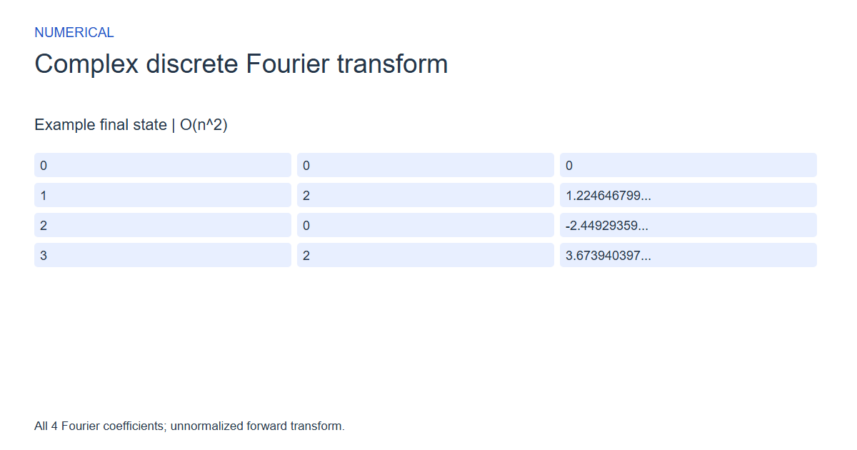
Step 20: All 4 Fourier coefficients; unnormalized forward transform.
State at this checkpoint
{
  "values": [
    0,
    0,
    0,
    1,
    2,
    1.2246467991473532e-16,
    2,
    0,
    -2.4492935982947064e-16,
    3,
    2,
    3.6739403974420594e-16
  ],
  "active": [],
  "kind": "matrix",
  "columns": 3,
  "columnLabels": [
    "k",
    "real",
    "imag"
  ],
  "rowLabels": [
    0,
    1,
    2,
    3
  ],
  "result": 4,
  "output": [
    0,
    0,
    2,
    1.2246467991473532e-16,
    0,
    -2.4492935982947064e-16,
    2,
    3.6739403974420594e-16
  ]
}
Expected final state
All 4 Fourier coefficients; unnormalized forward transform.
Complexity and input bounds
Family: Numerical. Time complexity: O(n^2).
Implementation detail: One through sixteen complex samples, real and imaginary components -9..9. Native empty DFT returns zero. Downloads return n and write 2*n interleaved real/imaginary doubles, preserving input arrays. Invalid length/direction returns -1 without output writes. Phasor frames show partial frequency sums and the final matrix lists every coefficient. An independent complex Horner oracle checks both directions with explicit tolerances.
Space complexity: O(1) auxiliary accumulation state excluding input/output and phasor frames.
Working-space bounds describe algorithm state and any explicitly noted output, excluding the visualization's saved timeline. Recording frames can use more memory than running the function alone. Here n is sequence length, V and E are vertex and edge counts, and other parameters refer to the named input dimensions.
1..16 complex samples real,imag separated by ;, then |0 forward or |1 inverse. Components -9..9. FFT requires a power-of-two length. Inverse divides by n.
The playground validates these limits before starting. Downloaded functions are callable implementations, with parameter and output-buffer contracts in their comments; they do not all repeat the playground's input validation.
Common mistakes and limitations
Do not discard imaginary components. Keep exponent sign and inverse normalization consistent. Nearly zero coefficients can contain floating-point roundoff.
Further reading
For background on algorithm analysis and the JavaScript function interface:
- MIT OpenCourseWare: algorithm design and analysis foundations
- MDN: JavaScript function parameters and return values
Editorial and testing approach · Browse all algorithm guides
Complete JavaScript implementation
1 2 3 4 5 | // Complex Fourier transform, components -9..9. Forward exponent is -2*pi*i*k*j/n; inverse flips the sign and divides by n. Output is 2*n interleaved real/imaginary doubles. Input arrays are unchanged. Return n or -1 invalid length/direction without output writes. DFT permits n 0..16 (empty returns 0); radix-2 FFT permits powers of two 1..16. Standard-library sin/cos, compare real results with explicit tolerances. DFT uses O(n^2) time and O(1) auxiliary numerical state. Reference snippets assume validated playground inputs. Fixed scratch buffers have 256 slots. Sorting variants may use a different traversal strategy than the animation. function algorithm(realInput, imagInput, n, inverse, output) { if (n < 0 || n > 16 || inverse < 0 || inverse > 1) { return -1; } let sign = -1.0; if (inverse == 1) { sign = 1.0; } let angle = 0.0; let cosine = 0.0; let sine = 0.0; let sumReal = 0.0; let sumImag = 0.0; let scale = 1.0; if (inverse == 1 && n > 0) { scale = 1.0/n; } for (let k = 0; k < n; k++) { sumReal = 0.0; sumImag = 0.0; for (let j = 0; j < n; j++) { angle = sign*6.283185307179586*k*j/n; cosine = Math.cos(angle); sine = Math.sin(angle); sumReal += realInput[j]*cosine-imagInput[j]*sine; sumImag += realInput[j]*sine+imagInput[j]*cosine; } output[2*k] = sumReal*scale; output[2*k+1] = sumImag*scale; } return n; } |
Source
Related primary research defines the complex discrete Fourier sums while developing a fast calculation. The playground DFT view evaluates those sums directly; this does not attribute the invention of the DFT to Cooley and Tukey.
- An algorithm for the machine calculation of complex Fourier series
James W. Cooley; John W. Tukey (1965). Research paper.