Published by Dimitris Kougioumtzis · Updated
Minimize weighted search cost over ordered keys, including frequencies for unsuccessful searches in every gap. Try each root for every interval.
For each ordered key interval, try every root and combine the optimal left and right costs. Adding the interval’s total successful and unsuccessful frequency accounts for making every subtree one level deeper.
When to use Optimal binary search tree
Building a static search tree when successful key frequencies and failed-search gap frequencies are known.
Choosing an alternative
Ordinary BST insertion depends on insertion order; AVL trees optimize height rather than a fixed query distribution. Knuth’s optimized recurrence reduces the cubic root search to quadratic time.
Worked example: input and state changes
Example input
15,10,5,10,20 | 5,10,5,5,5,10These checkpoints follow the actual example timeline. State details show the stored values and decisions; use the visualization to inspect every intervening step.
Step 0: Empty intervals cost their gap frequency. Root depth is one; unsuccessful leaf depth is counted too.
State at this checkpoint
{
  "values": [
    5,
    0,
    0,
    0,
    0,
    0,
    0,
    10,
    0,
    0,
    0,
    0,
    0,
    0,
    5,
    0,
    0,
    0,
    0,
    0,
    0,
    5,
    0,
    0,
    0,
    0,
    0,
    0,
    5,
    0,
    0,
    0,
    0,
    0,
    0,
    10
  ],
  "active": [],
  "kind": "matrix",
  "columns": 6,
  "roots": [
    -1,
    -1,
    -1,
    -1,
    -1,
    -1,
    -1,
    -1,
    -1,
    -1,
    -1,
    -1,
    -1,
    -1,
    -1,
    -1,
    -1,
    -1,
    -1,
    -1,
    -1,
    -1,
    -1,
    -1,
    -1,
    -1,
    -1,
    -1,
    -1,
    -1,
    -1,
    -1,
    -1,
    -1,
    -1,
    -1
  ]
}
Step 6: Keys 0..1: root 0 gives weighted cost 90.
State at this checkpoint
{
  "values": [
    5,
    45,
    90,
    0,
    0,
    0,
    0,
    10,
    40,
    0,
    0,
    0,
    0,
    0,
    5,
    25,
    0,
    0,
    0,
    0,
    0,
    5,
    30,
    0,
    0,
    0,
    0,
    0,
    5,
    50,
    0,
    0,
    0,
    0,
    0,
    10
  ],
  "active": [
    2
  ],
  "kind": "matrix",
  "columns": 6,
  "roots": [
    -1,
    0,
    0,
    -1,
    -1,
    -1,
    -1,
    -1,
    1,
    -1,
    -1,
    -1,
    -1,
    -1,
    -1,
    2,
    -1,
    -1,
    -1,
    -1,
    -1,
    -1,
    3,
    -1,
    -1,
    -1,
    -1,
    -1,
    -1,
    4,
    -1,
    -1,
    -1,
    -1,
    -1,
    -1
  ]
}
Step 13: Keys 0..2: root 1 gives weighted cost 125.
State at this checkpoint
{
  "values": [
    5,
    45,
    90,
    125,
    0,
    0,
    0,
    10,
    40,
    70,
    0,
    0,
    0,
    0,
    5,
    25,
    60,
    0,
    0,
    0,
    0,
    5,
    30,
    90,
    0,
    0,
    0,
    0,
    5,
    50,
    0,
    0,
    0,
    0,
    0,
    10
  ],
  "active": [
    3
  ],
  "kind": "matrix",
  "columns": 6,
  "roots": [
    -1,
    0,
    0,
    1,
    -1,
    -1,
    -1,
    -1,
    1,
    1,
    -1,
    -1,
    -1,
    -1,
    -1,
    2,
    3,
    -1,
    -1,
    -1,
    -1,
    -1,
    3,
    4,
    -1,
    -1,
    -1,
    -1,
    -1,
    4,
    -1,
    -1,
    -1,
    -1,
    -1,
    -1
  ]
}
Step 19: Keys 0..3: root 1 gives weighted cost 175.
State at this checkpoint
{
  "values": [
    5,
    45,
    90,
    125,
    175,
    0,
    0,
    10,
    40,
    70,
    120,
    0,
    0,
    0,
    5,
    25,
    60,
    130,
    0,
    0,
    0,
    5,
    30,
    90,
    0,
    0,
    0,
    0,
    5,
    50,
    0,
    0,
    0,
    0,
    0,
    10
  ],
  "active": [
    4
  ],
  "kind": "matrix",
  "columns": 6,
  "roots": [
    -1,
    0,
    0,
    1,
    1,
    -1,
    -1,
    -1,
    1,
    1,
    1,
    -1,
    -1,
    -1,
    -1,
    2,
    3,
    4,
    -1,
    -1,
    -1,
    -1,
    3,
    4,
    -1,
    -1,
    -1,
    -1,
    -1,
    4,
    -1,
    -1,
    -1,
    -1,
    -1,
    -1
  ]
}
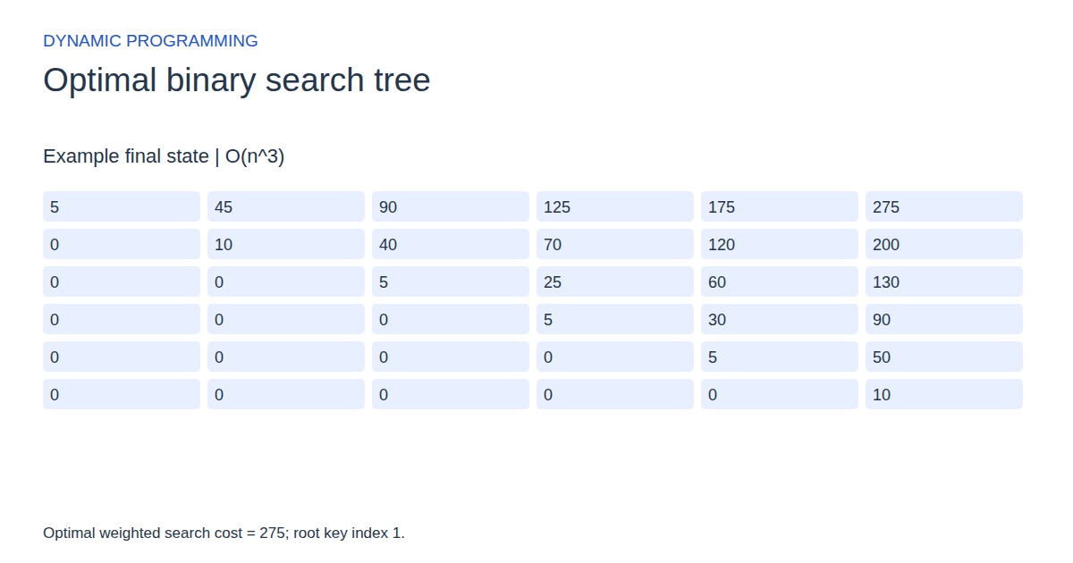
Step 25: Optimal weighted search cost = 275; root key index 1.
State at this checkpoint
{
  "values": [
    5,
    45,
    90,
    125,
    175,
    275,
    0,
    10,
    40,
    70,
    120,
    200,
    0,
    0,
    5,
    25,
    60,
    130,
    0,
    0,
    0,
    5,
    30,
    90,
    0,
    0,
    0,
    0,
    5,
    50,
    0,
    0,
    0,
    0,
    0,
    10
  ],
  "active": [],
  "kind": "matrix",
  "columns": 6,
  "roots": [
    -1,
    0,
    0,
    1,
    1,
    1,
    -1,
    -1,
    1,
    1,
    1,
    3,
    -1,
    -1,
    -1,
    2,
    3,
    4,
    -1,
    -1,
    -1,
    -1,
    3,
    4,
    -1,
    -1,
    -1,
    -1,
    -1,
    4,
    -1,
    -1,
    -1,
    -1,
    -1,
    -1
  ],
  "result": 275,
  "root": 1
}
Expected final state
Optimal weighted search cost = 275; root key index 1.
Complexity and input bounds
Family: Dynamic programming. Time complexity: O(n^3).
Implementation detail: This bounded view uses the straightforward O(n^3) dynamic program, not the O(n^2) root-monotonicity optimization. Matrix cell [i,j] describes half-open key interval [i,j). Downloads write a complete root table; equal-cost roots choose the smallest index. An empty download input returns its only gap frequency.
Space complexity: O(n^2) auxiliary storage for interval costs, weights and root choices, excluding saved visualization frames.
Working-space bounds describe algorithm state and any explicitly noted output, excluding the visualization's saved timeline. Recording frames can use more memory than running the function alone. Here n is sequence length, V and E are vertex and edge counts, and other parameters refer to the named input dimensions.
1..8 successful-search frequencies p | n+1 unsuccessful-search frequencies q. Integers 0..99; key order is fixed.
The playground validates these limits before starting. Downloaded functions are callable implementations, with parameter and output-buffer contracts in their comments; they do not all repeat the playground's input validation.
Common mistakes and limitations
Keys remain in sorted order; only the shape changes. Include all n+1 failed-search gaps. Root and external failed-search leaves have depth counted from one. Do not confuse raw weighted cost with a normalized expectation.
Further reading
For background on algorithm analysis and the JavaScript function interface:
- MIT OpenCourseWare: algorithm design and analysis foundations
- MDN: JavaScript function parameters and return values
Editorial and testing approach · Browse all algorithm guides
Complete JavaScript implementation
1 2 3 4 5 6 7 8 9 10 11 12 13 14 15 16 | // Ordered keys: n 0..8; p has n successful frequencies and q has n+1 failed-search gap frequencies, all 0..99. Root depth 1; external failed-search leaves also contribute frequency times depth. Returns minimum weighted cost (not normalized probability). Writes (n+1)^2 root indices for half-open intervals [i,j) row-major; empty/unused cells -1, ties choose the smallest root. Output capacity at least (n+1)^2. Empty tree returns q[0]. O(n^3) time, O(n^2) auxiliary space; this does not use Knuth's O(n^2) optimization. Reference snippets assume validated playground inputs. Fixed scratch buffers have 256 slots. Sorting variants may use a different traversal strategy than the animation. function algorithm(p, q, n, output) { let cost = Array(256).fill(0); let weight = Array(256).fill(0); let s = n + 1; let j = 0; let candidate = 0; for (let i = 0; i < s * s; i++) { output[i] = -1; } for (let i = 0; i <= n; i++) { cost[i * s + i] = q[i]; weight[i * s + i] = q[i]; } for (let length = 1; length <= n; length++) { for (let i = 0; i + length <= n; i++) { j = i + length; weight[i * s + j] = weight[i * s + j - 1] + p[j - 1] + q[j]; cost[i * s + j] = 1000000; for (let r = i; r < j; r++) { candidate = cost[i * s + r] + cost[(r + 1) * s + j] + weight[i * s + j]; if (candidate < cost[i * s + j]) { cost[i * s + j] = candidate; output[i * s + j] = r; } } } } return cost[n]; } |
Source
Primary research on optimum binary search trees and root-choice optimization. The playground uses the straightforward cubic interval recurrence, not the paper’s quadratic optimization.
- Optimum binary search trees
Donald E. Knuth (1971). Research paper.