Published by Dimitris Kougioumtzis · Updated
Insert keys, delete a key, insert another key, then search. Resolve collisions by linear probing; tombstones preserve search paths.
Probe successive slots from key modulo 17. Tombstones preserve collision chains after deletion. Insert initial keys, delete a key, insert one more key, then search the final set.
When to use Hash table linear probing
Teaching collision resolution, duplicate suppression, deletion and reinsertion in bounded hash sets.
Choosing an alternative
Separate chaining uses linked records. Linear probing can cluster; quadratic and double hashing change the probe sequence.
Worked example: input and state changes
Example input
1,18,35,52,69 | 18,86,35These checkpoints follow the actual example timeline. State details show the stored values and decisions; use the visualization to inspect every intervening step.
Step 0: Initialize 17 empty slots.
State at this checkpoint
{
  "values": [
    "empty",
    "empty",
    "empty",
    "empty",
    "empty",
    "empty",
    "empty",
    "empty",
    "empty",
    "empty",
    "empty",
    "empty",
    "empty",
    "empty",
    "empty",
    "empty",
    "empty"
  ],
  "active": [],
  "kind": "matrix",
  "columns": 4
}
Step 9: Place a new key or retain an existing duplicate.
State at this checkpoint
{
  "values": [
    "empty",
    1,
    18,
    35,
    "empty",
    "empty",
    "empty",
    "empty",
    "empty",
    "empty",
    "empty",
    "empty",
    "empty",
    "empty",
    "empty",
    "empty",
    "empty"
  ],
  "active": [
    3
  ],
  "kind": "matrix",
  "columns": 4
}
Step 17: Insert 69: probe 2, slot 3.
State at this checkpoint
{
  "values": [
    "empty",
    1,
    18,
    35,
    52,
    "empty",
    "empty",
    "empty",
    "empty",
    "empty",
    "empty",
    "empty",
    "empty",
    "empty",
    "empty",
    "empty",
    "empty"
  ],
  "active": [
    3
  ],
  "kind": "matrix",
  "columns": 4
}
Step 26: Insert 86: probe 2, slot 3.
State at this checkpoint
{
  "values": [
    "empty",
    1,
    "deleted",
    35,
    52,
    69,
    "empty",
    "empty",
    "empty",
    "empty",
    "empty",
    "empty",
    "empty",
    "empty",
    "empty",
    "empty",
    "empty"
  ],
  "active": [
    3
  ],
  "kind": "matrix",
  "columns": 4
}
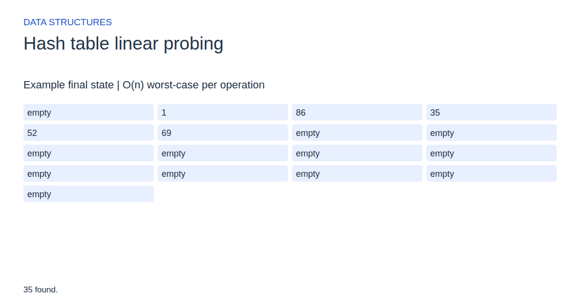
Step 34: 35 found.
State at this checkpoint
{
  "values": [
    "empty",
    1,
    86,
    35,
    52,
    69,
    "empty",
    "empty",
    "empty",
    "empty",
    "empty",
    "empty",
    "empty",
    "empty",
    "empty",
    "empty",
    "empty"
  ],
  "active": [],
  "kind": "matrix",
  "columns": 4,
  "result": 1
}
Expected final state
35 found.
Complexity and input bounds
Family: Data structures. Time complexity: O(n) worst-case per operation.
Implementation detail: There are seventeen buckets or slots, keys 0..99, at most seven initial keys and one later insertion. At most eight live keys keep the load below one half, including for the triangular quadratic probe variant. Downloads return membership and serialize the table, sorted keys and comparison count. Individual operations are linear in the worst case; the reporting pass scans the bounded key universe.
Space complexity: O(n + table capacity + key universe) auxiliary storage, including bounded serialization helpers; animation frames use additional space.
Working-space bounds describe algorithm state and any explicitly noted output, excluding the visualization's saved timeline. Recording frames can use more memory than running the function alone. Here n is sequence length, V and E are vertex and edge counts, and other parameters refer to the named input dimensions.
1..7 initial keys | delete,insert,search keys. Keys 0..99; 17 buckets/slots; duplicate keys ignored.
The playground validates these limits before starting. Downloaded functions are callable implementations, with parameter and output-buffer contracts in their comments; they do not all repeat the playground's input validation.
Common mistakes and limitations
Do not replace a deleted slot with an empty marker: that can hide later colliding keys. Continue searching across tombstones before declaring a key absent.
Further reading
For background on algorithm analysis and the JavaScript function interface:
- MIT OpenCourseWare: algorithm design and analysis foundations
- MDN: JavaScript function parameters and return values
Editorial and testing approach · Browse all algorithm guides
Complete JavaScript implementation
1 2 3 4 5 6 7 8 9 10 11 12 13 14 15 16 17 18 19 20 21 22 23 24 25 26 27 28 29 30 | // Hash set: n 0..7 initial keys, all keys/deleteKey/insertKey/target 0..99. Insert initial keys, delete once, insert once, then return target membership. Duplicate keys ignored. 17 buckets/slots; at most 8 live keys. Empty=-1, tombstone=-2. Linear offsets 0..16. Output capacity at least 132: [0..16] slot values/bucket heads; [17] count; [18..25] sorted keys; [26] search comparisons. Chaining additionally writes [32+key] next key (-1 chain end, -2 absent); these cells are zero for probing. Operations are O(n) worst case; bounded serialization scans the 100-key universe. Auxiliary space O(n + table capacity + key universe). Reference snippets assume validated playground inputs. Fixed scratch buffers have 256 slots. Sorting variants may use a different traversal strategy than the animation. function algorithm(a, n, deleteKey, insertKey, target, output) { let present = Array(256).fill(0); let table = Array(256).fill(0); let probe = 0; let slot = 0; let tomb = 0; let value = 0; let deleting = 0; let found = 0; let length = 0; let comparisons = 0; for (let i = 0; i < 17; i++) { table[i] = -1; } for (let operation = 0; operation < n + 2; operation++) { deleting = 0; value = insertKey; if (operation < n) { value = a[operation]; } else if (operation == n) { value = deleteKey; deleting = 1; } tomb = -1; found = 0; for (probe = 0; probe < 17; probe++) { slot = (value % 17 + probe) % 17; if (table[slot] == value) { found = 1; break; } if (table[slot] == -2 && tomb < 0) { tomb = slot; } if (table[slot] == -1) { break; } } if (deleting != 0 && found != 0) { table[slot] = -2; present[value] = 0; } else if (deleting == 0 && found == 0) { if (tomb >= 0) { slot = tomb; } else if (probe == 17) { return -2; } table[slot] = value; present[value] = 1; } } found = 0; value = target; for (probe = 0; probe < 17; probe++) { slot = (value % 17 + probe) % 17; comparisons++; if (table[slot] == value) { found = 1; break; } if (table[slot] == -1) { break; } } for (let i = 0; i < 132; i++) { output[i] = 0; } for (let i = 0; i < 17; i++) { output[i] = table[i]; } for (let i = 0; i < 100; i++) { if (present[i] != 0) { output[18 + length++] = i; } } output[17] = length; output[26] = comparisons; return found; } |
Source
Authoritative authored book reference for hashing and collision-resolution methods. No original research paper for this exact bounded variant has been verified; the playground fixes capacity, hash formulas and operation order for reproducible comparison.
- The Art of Computer Programming, Volume 3: Sorting and Searching (2nd edition)
Donald E. Knuth (1998). Reference book.