Published by Dimitris Kougioumtzis · Updated
Transform bounded complex samples into Fourier coefficients, or apply the normalized inverse transform.
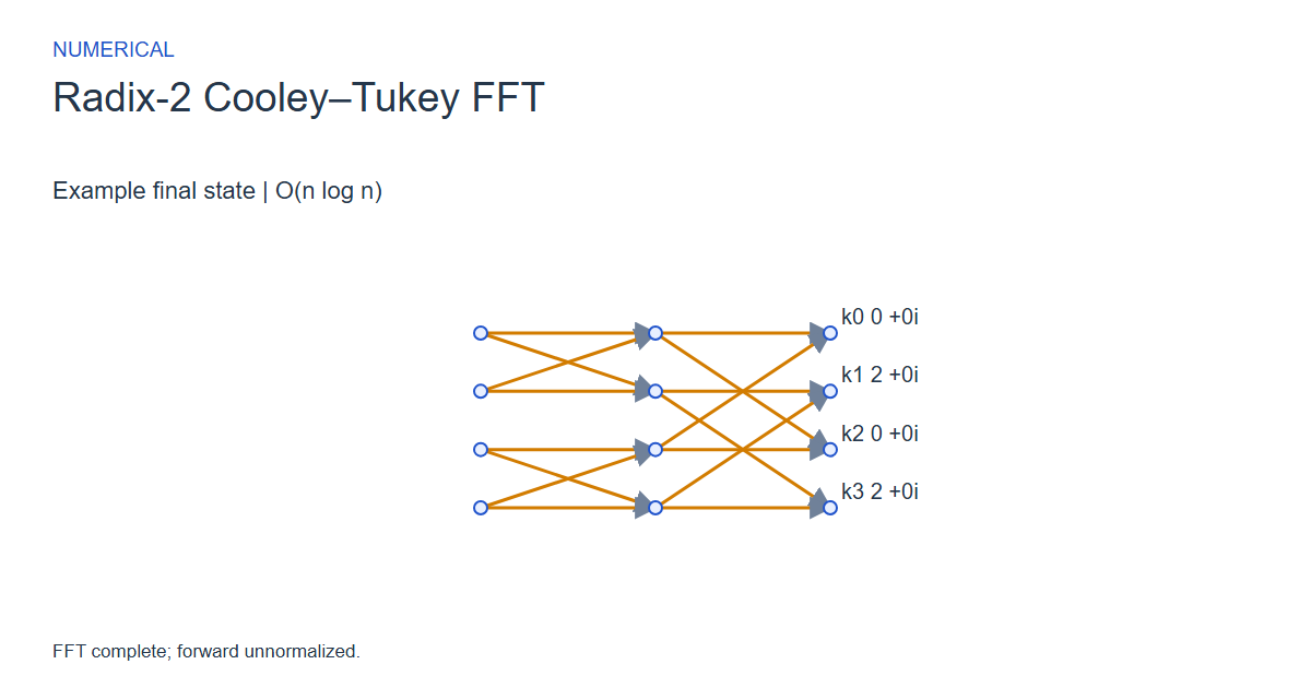
Reorder samples by reversed binary indices, then combine pairs through width-two, four and larger butterfly stages. Each butterfly rotates one input by a twiddle factor and produces its sum and difference with the other input.
When to use Radix-2 Cooley–Tukey FFT
Learning how Fourier factorization reuses work and connects a staged butterfly network to complex frequency coefficients.
Choosing an alternative
Direct DFT takes O(n^2) work. This radix-two Cooley-Tukey implementation takes O(n log n) and requires a power-of-two length; it does not implement mixed-radix or arbitrary-length FFT planning.
Worked example: input and state changes
Example input
1,0;0,0;-1,0;0,0|0These checkpoints follow the actual example timeline. State details show the stored values and decisions; use the visualization to inspect every intervening step.
Step 0: Bit-reverse input indices; stages run left to right.
State at this checkpoint
{
  "values": [
    "k0 1 +0i",
    "k1 -1 +0i",
    "k2 0 +0i",
    "k3 0 +0i",
    "pending",
    "pending",
    "pending",
    "pending",
    "pending",
    "pending",
    "pending",
    "pending"
  ],
  "active": [],
  "kind": "graph",
  "points": [
    [
      0,
      3
    ],
    [
      0,
      2
    ],
    [
      0,
      1
    ],
    [
      0,
      0
    ],
    [
      3,
      3
    ],
    [
      3,
      2
    ],
    [
      3,
      1
    ],
    [
      3,
      0
    ],
    [
      6,
      3
    ],
    [
      6,
      2
    ],
    [
      6,
      1
    ],
    [
      6,
      0
    ]
  ],
  "nodeLabels": [
    "k0 1 +0i",
    "k1 -1 +0i",
    "k2 0 +0i",
    "k3 0 +0i",
    "pending",
    "pending",
    "pending",
    "pending",
    "pending",
    "pending",
    "pending",
    "pending"
  ],
  "pointMarkerIndices": [
    0,
    1,
    2,
    3
  ],
  "pointLabelIndices": [
    0
  ],
  "directed": true,
  "chosen": [],
  "visited": [],
  "result": 0,
  "output": []
}
Step 1: Stage 1, width 2: butterfly 0 / 1.
State at this checkpoint
{
  "values": [
    "k0 1 +0i",
    "k1 -1 +0i",
    "k2 0 +0i",
    "k3 0 +0i",
    "k0 0 +0i",
    "k1 2 +0i",
    "pending",
    "pending",
    "pending",
    "pending",
    "pending",
    "pending"
  ],
  "active": [
    4,
    5
  ],
  "kind": "graph",
  "points": [
    [
      0,
      3
    ],
    [
      0,
      2
    ],
    [
      0,
      1
    ],
    [
      0,
      0
    ],
    [
      3,
      3
    ],
    [
      3,
      2
    ],
    [
      3,
      1
    ],
    [
      3,
      0
    ],
    [
      6,
      3
    ],
    [
      6,
      2
    ],
    [
      6,
      1
    ],
    [
      6,
      0
    ]
  ],
  "nodeLabels": [
    "k0 1 +0i",
    "k1 -1 +0i",
    "k2 0 +0i",
    "k3 0 +0i",
    "k0 0 +0i",
    "k1 2 +0i",
    "pending",
    "pending",
    "pending",
    "pending",
    "pending",
    "pending"
  ],
  "pointMarkerIndices": [
    0,
    1,
    2,
    3,
    4,
    5
  ],
  "pointLabelIndices": [
    4,
    5
  ],
  "directed": true,
  "chosen": [
    0,
    1,
    2,
    3
  ],
  "visited": [],
  "result": 0,
  "output": []
}
Step 3: Stage 2, width 4: butterfly 0 / 2.
State at this checkpoint
{
  "values": [
    "k0 1 +0i",
    "k1 -1 +0i",
    "k2 0 +0i",
    "k3 0 +0i",
    "k0 0 +0i",
    "k1 2 +0i",
    "k2 0 +0i",
    "k3 0 +0i",
    "k0 0 +0i",
    "pending",
    "k2 0 +0i",
    "pending"
  ],
  "active": [
    8,
    10
  ],
  "kind": "graph",
  "points": [
    [
      0,
      3
    ],
    [
      0,
      2
    ],
    [
      0,
      1
    ],
    [
      0,
      0
    ],
    [
      3,
      3
    ],
    [
      3,
      2
    ],
    [
      3,
      1
    ],
    [
      3,
      0
    ],
    [
      6,
      3
    ],
    [
      6,
      2
    ],
    [
      6,
      1
    ],
    [
      6,
      0
    ]
  ],
  "nodeLabels": [
    "k0 1 +0i",
    "k1 -1 +0i",
    "k2 0 +0i",
    "k3 0 +0i",
    "k0 0 +0i",
    "k1 2 +0i",
    "k2 0 +0i",
    "k3 0 +0i",
    "k0 0 +0i",
    "pending",
    "k2 0 +0i",
    "pending"
  ],
  "pointMarkerIndices": [
    0,
    1,
    2,
    3,
    4,
    5,
    6,
    7,
    8,
    10
  ],
  "pointLabelIndices": [
    8,
    10
  ],
  "directed": true,
  "chosen": [
    0,
    1,
    2,
    3,
    4,
    5,
    6,
    7,
    8,
    9,
    10,
    11
  ],
  "visited": [],
  "result": 0,
  "output": []
}
Step 4: Stage 2, width 4: butterfly 1 / 3.
State at this checkpoint
{
  "values": [
    "k0 1 +0i",
    "k1 -1 +0i",
    "k2 0 +0i",
    "k3 0 +0i",
    "k0 0 +0i",
    "k1 2 +0i",
    "k2 0 +0i",
    "k3 0 +0i",
    "k0 0 +0i",
    "k1 2 +0i",
    "k2 0 +0i",
    "k3 2 +0i"
  ],
  "active": [
    9,
    11
  ],
  "kind": "graph",
  "points": [
    [
      0,
      3
    ],
    [
      0,
      2
    ],
    [
      0,
      1
    ],
    [
      0,
      0
    ],
    [
      3,
      3
    ],
    [
      3,
      2
    ],
    [
      3,
      1
    ],
    [
      3,
      0
    ],
    [
      6,
      3
    ],
    [
      6,
      2
    ],
    [
      6,
      1
    ],
    [
      6,
      0
    ]
  ],
  "nodeLabels": [
    "k0 1 +0i",
    "k1 -1 +0i",
    "k2 0 +0i",
    "k3 0 +0i",
    "k0 0 +0i",
    "k1 2 +0i",
    "k2 0 +0i",
    "k3 0 +0i",
    "k0 0 +0i",
    "k1 2 +0i",
    "k2 0 +0i",
    "k3 2 +0i"
  ],
  "pointMarkerIndices": [
    0,
    1,
    2,
    3,
    4,
    5,
    6,
    7,
    8,
    9,
    10,
    11
  ],
  "pointLabelIndices": [
    9,
    11
  ],
  "directed": true,
  "chosen": [
    0,
    1,
    2,
    3,
    4,
    5,
    6,
    7,
    8,
    9,
    10,
    11,
    12,
    13,
    14,
    15
  ],
  "visited": [],
  "result": 0,
  "output": []
}
Step 5: FFT complete; forward unnormalized.
State at this checkpoint
{
  "values": [
    "k0 1 +0i",
    "k1 -1 +0i",
    "k2 0 +0i",
    "k3 0 +0i",
    "k0 0 +0i",
    "k1 2 +0i",
    "k2 0 +0i",
    "k3 0 +0i",
    "k0 0 +0i",
    "k1 2 +0i",
    "k2 0 +0i",
    "k3 2 +0i"
  ],
  "active": [],
  "kind": "graph",
  "points": [
    [
      0,
      3
    ],
    [
      0,
      2
    ],
    [
      0,
      1
    ],
    [
      0,
      0
    ],
    [
      3,
      3
    ],
    [
      3,
      2
    ],
    [
      3,
      1
    ],
    [
      3,
      0
    ],
    [
      6,
      3
    ],
    [
      6,
      2
    ],
    [
      6,
      1
    ],
    [
      6,
      0
    ]
  ],
  "nodeLabels": [
    "k0 1 +0i",
    "k1 -1 +0i",
    "k2 0 +0i",
    "k3 0 +0i",
    "k0 0 +0i",
    "k1 2 +0i",
    "k2 0 +0i",
    "k3 0 +0i",
    "k0 0 +0i",
    "k1 2 +0i",
    "k2 0 +0i",
    "k3 2 +0i"
  ],
  "pointMarkerIndices": [
    0,
    1,
    2,
    3,
    4,
    5,
    6,
    7,
    8,
    9,
    10,
    11
  ],
  "pointLabelIndices": [
    8,
    9,
    10,
    11
  ],
  "directed": true,
  "chosen": [
    0,
    1,
    2,
    3,
    4,
    5,
    6,
    7,
    8,
    9,
    10,
    11,
    12,
    13,
    14,
    15
  ],
  "visited": [],
  "result": 4,
  "output": [
    0,
    0,
    2,
    0,
    0,
    0,
    2,
    0
  ]
}
Expected final state
FFT complete; forward unnormalized.
Complexity and input bounds
Family: Numerical. Time complexity: O(n log n).
Implementation detail: Power-of-two sample counts one through sixteen, components -9..9. Downloads return n and write interleaved complex coefficients; inverse flips exponent sign and divides by n. Invalid parameters return -1 without output writes. Portable versions use iterative bit-reversed butterflies; Python independently uses recursive even/odd decomposition. The WebGL and 2D network reveals only computed stage nodes. Independent Horner fixtures check every output in both directions.
Space complexity: O(n) complex working values excluding input/output and network frames.
Working-space bounds describe algorithm state and any explicitly noted output, excluding the visualization's saved timeline. Recording frames can use more memory than running the function alone. Here n is sequence length, V and E are vertex and edge counts, and other parameters refer to the named input dimensions.
1..16 complex samples real,imag separated by ;, then |0 forward or |1 inverse. Components -9..9. FFT requires a power-of-two length. Inverse divides by n.
The playground validates these limits before starting. Downloaded functions are callable implementations, with parameter and output-buffer contracts in their comments; they do not all repeat the playground's input validation.
Common mistakes and limitations
Read both butterfly inputs before overwriting either output. Reverse the required number of index bits and apply inverse normalization exactly once. Pending stage nodes must not look completed.
Further reading
For background on algorithm analysis and the JavaScript function interface:
- MIT OpenCourseWare: algorithm design and analysis foundations
- MDN: JavaScript function parameters and return values
Editorial and testing approach · Browse all algorithm guides
Complete JavaScript implementation
1 2 3 4 5 6 7 8 | // Complex Fourier transform, components -9..9. Forward exponent is -2*pi*i*k*j/n; inverse flips the sign and divides by n. Output is 2*n interleaved real/imaginary doubles. Input arrays are unchanged. Return n or -1 invalid length/direction without output writes. DFT permits n 0..16 (empty returns 0); radix-2 FFT permits powers of two 1..16. Standard-library sin/cos, compare real results with explicit tolerances. Iterative bit-reversed Cooley-Tukey butterflies use O(n log n) time and O(n) working arrays; the Python implementation uses recursive even/odd splitting. Reference snippets assume validated playground inputs. Fixed scratch buffers have 256 slots. Sorting variants may use a different traversal strategy than the animation. function algorithm(realInput, imagInput, n, inverse, output) { if (n < 1 || n > 16 || (n&(n-1)) != 0 || inverse < 0 || inverse > 1) { return -1; } let workReal = Array(256).fill(0); let workImag = Array(256).fill(0); let reversed = 0; let value = 0; let bits = 0; let half = 0; let first = 0; let second = 0; let sign = -1.0; if (inverse == 1) { sign = 1.0; } let angle = 0.0; let cosine = 0.0; let sine = 0.0; let tr = 0.0; let ti = 0.0; let ar = 0.0; let ai = 0.0; let scale = 1.0; for (let i = 0; i < n; i++) { reversed = 0; value = i; bits = n>>1; while (bits > 0) { reversed = 2*reversed+(value&1); value >>= 1; bits >>= 1; } workReal[reversed] = realInput[i]; workImag[reversed] = imagInput[i]; } for (let width = 2; width <= n; width *= 2) { half = width>>1; for (let start = 0; start < n; start += width) { for (let j = 0; j < half; j++) { first = start+j; second = first+half; angle = sign*6.283185307179586*j/width; cosine = Math.cos(angle); sine = Math.sin(angle); tr = cosine*workReal[second]-sine*workImag[second]; ti = cosine*workImag[second]+sine*workReal[second]; ar = workReal[first]; ai = workImag[first]; workReal[first] = ar+tr; workImag[first] = ai+ti; workReal[second] = ar-tr; workImag[second] = ai-ti; } } } if (inverse == 1) { scale = 1.0/n; } for (let i = 0; i < n; i++) { output[2*i] = workReal[i]*scale; output[2*i+1] = workImag[i]*scale; } return n; } |
Source
Foundational fast Fourier transform research. The playground specializes the factorization to bounded radix-two complex transforms with explicit bit-reversed iteration and normalized inverse convention.
- An algorithm for the machine calculation of complex Fourier series
James W. Cooley; John W. Tukey (1965). Research paper.