Published by Dimitris Kougioumtzis · Updated
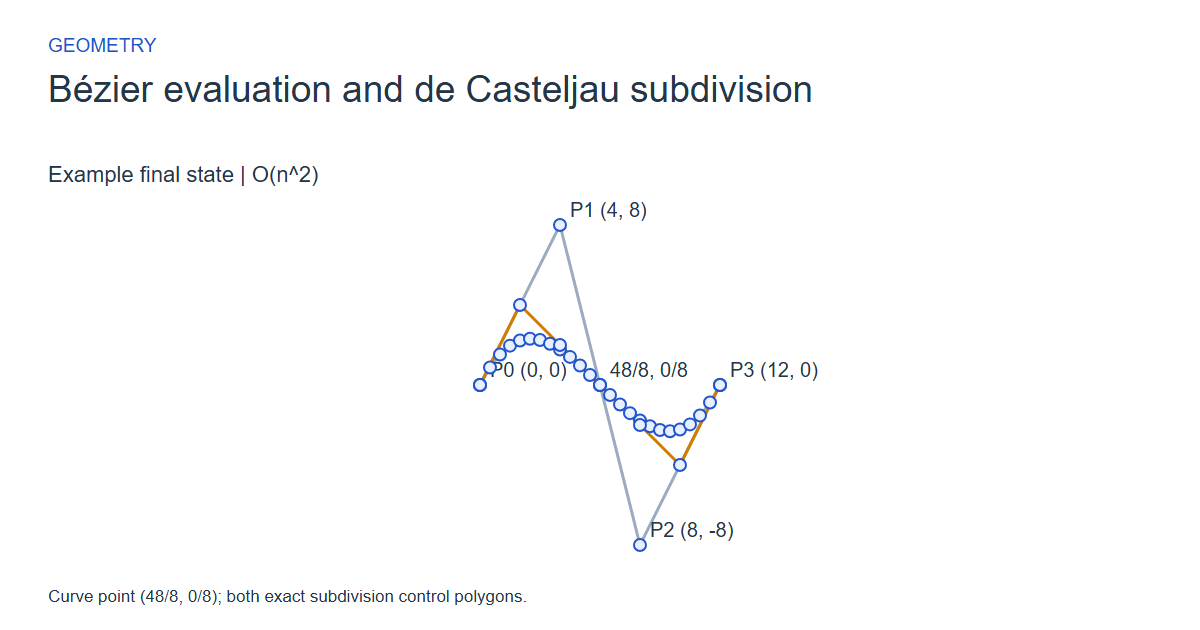
Interpolate adjacent control points repeatedly to evaluate a Bézier curve and construct both subdivision control polygons.
Interpolate adjacent control points at the same parameter repeatedly until one point remains. The left and right edges of this interpolation triangle become the control polygons for the two subdivided curve segments.
When to use Bézier evaluation and de Casteljau subdivision
Evaluating and splitting Bezier curves in vector drawing, animation paths and geometric design.
Choosing an alternative
Bernstein evaluation forms a weighted sum directly. De Casteljau builds a geometric interpolation triangle that also supplies both subdivision polygons. The fixture oracle uses independent Bernstein sums rather than repeating the product recurrence.
Worked example: input and state changes
Example input
0,0;4,8;8,-8;12,0|1,2These checkpoints follow the actual example timeline. State details show the stored values and decisions; use the visualization to inspect every intervening step.
Step 0: Level 0: denominator 1; interpolate with t=1/2.
State at this checkpoint
{
  "values": [
    0,
    1,
    2,
    3,
    4,
    5,
    6,
    7,
    8,
    9,
    10,
    11,
    12,
    13,
    14,
    15,
    16,
    17,
    18,
    19,
    20,
    21,
    22,
    23,
    24,
    25,
    26,
    27,
    28,
    29,
    30,
    31,
    32
  ],
  "active": [],
  "kind": "graph",
  "points": [
    [
      0,
      0
    ],
    [
      4,
      8
    ],
    [
      8,
      -8
    ],
    [
      12,
      0
    ],
    [
      0,
      0
    ],
    [
      0.5,
      0.8784722222222223
    ],
    [
      0.9999999999999998,
      1.5277777777777775
    ],
    [
      1.5,
      1.96875
    ],
    [
      2.0000000000000004,
      2.2222222222222223
    ],
    [
      2.5,
      2.3090277777777777
    ],
    [
      3,
      2.25
    ],
    [
      3.4999999999999996,
      2.065972222222222
    ],
    [
      4,
      1.7777777777777783
    ],
    [
      4.5,
      1.40625
    ],
    [
      4.999999999999999,
      0.9722222222222215
    ],
    [
      5.500000000000001,
      0.49652777777777857
    ],
    [
      6,
      0
    ],
    [
      6.5,
      -0.49652777777777724
    ],
    [
      7,
      -0.9722222222222225
    ],
    [
      7.5,
      -1.40625
    ],
    [
      8,
      -1.7777777777777777
    ],
    [
      8.5,
      -2.0659722222222223
    ],
    [
      9,
      -2.25
    ],
    [
      9.5,
      -2.3090277777777777
    ],
    [
      10,
      -2.2222222222222223
    ],
    [
      10.5,
      -1.96875
    ],
    [
      11,
      -1.5277777777777783
    ],
    [
      11.5,
      -0.8784722222222217
    ],
    [
      12,
      0
    ],
    [
      0,
      0
    ],
    [
      4,
      8
    ],
    [
      8,
      -8
    ],
    [
      12,
      0
    ]
  ],
  "nodeLabels": [
    "P0 (0, 0)",
    "P1 (4, 8)",
    "P2 (8, -8)",
    "P3 (12, 0)",
    "",
    "",
    "",
    "",
    "",
    "",
    "",
    "",
    "",
    "",
    "",
    "",
    "",
    "",
    "",
    "",
    "",
    "",
    "",
    "",
    "",
    "",
    "",
    "",
    "",
    "0/1, 0/1",
    "4/1, 8/1",
    "8/1, -8/1",
    "12/1, 0/1"
  ],
  "pointLabelIndices": [
    0,
    1,
    2,
    3
  ],
  "directed": false,
  "chosen": [
    27,
    28,
    29
  ],
  "visited": [],
  "result": 0,
  "output": []
}
Step 1: Level 1: denominator 2; interpolate with t=1/2.
State at this checkpoint
{
  "values": [
    0,
    1,
    2,
    3,
    4,
    5,
    6,
    7,
    8,
    9,
    10,
    11,
    12,
    13,
    14,
    15,
    16,
    17,
    18,
    19,
    20,
    21,
    22,
    23,
    24,
    25,
    26,
    27,
    28,
    29,
    30,
    31
  ],
  "active": [],
  "kind": "graph",
  "points": [
    [
      0,
      0
    ],
    [
      4,
      8
    ],
    [
      8,
      -8
    ],
    [
      12,
      0
    ],
    [
      0,
      0
    ],
    [
      0.5,
      0.8784722222222223
    ],
    [
      0.9999999999999998,
      1.5277777777777775
    ],
    [
      1.5,
      1.96875
    ],
    [
      2.0000000000000004,
      2.2222222222222223
    ],
    [
      2.5,
      2.3090277777777777
    ],
    [
      3,
      2.25
    ],
    [
      3.4999999999999996,
      2.065972222222222
    ],
    [
      4,
      1.7777777777777783
    ],
    [
      4.5,
      1.40625
    ],
    [
      4.999999999999999,
      0.9722222222222215
    ],
    [
      5.500000000000001,
      0.49652777777777857
    ],
    [
      6,
      0
    ],
    [
      6.5,
      -0.49652777777777724
    ],
    [
      7,
      -0.9722222222222225
    ],
    [
      7.5,
      -1.40625
    ],
    [
      8,
      -1.7777777777777777
    ],
    [
      8.5,
      -2.0659722222222223
    ],
    [
      9,
      -2.25
    ],
    [
      9.5,
      -2.3090277777777777
    ],
    [
      10,
      -2.2222222222222223
    ],
    [
      10.5,
      -1.96875
    ],
    [
      11,
      -1.5277777777777783
    ],
    [
      11.5,
      -0.8784722222222217
    ],
    [
      12,
      0
    ],
    [
      2,
      4
    ],
    [
      6,
      0
    ],
    [
      10,
      -4
    ]
  ],
  "nodeLabels": [
    "P0 (0, 0)",
    "P1 (4, 8)",
    "P2 (8, -8)",
    "P3 (12, 0)",
    "",
    "",
    "",
    "",
    "",
    "",
    "",
    "",
    "",
    "",
    "",
    "",
    "",
    "",
    "",
    "",
    "",
    "",
    "",
    "",
    "",
    "",
    "",
    "",
    "",
    "4/2, 8/2",
    "12/2, 0/2",
    "20/2, -8/2"
  ],
  "pointLabelIndices": [
    0,
    1,
    2,
    3
  ],
  "directed": false,
  "chosen": [
    27,
    28
  ],
  "visited": [],
  "result": 1,
  "output": []
}
Step 2: Level 2: denominator 4; interpolate with t=1/2.
State at this checkpoint
{
  "values": [
    0,
    1,
    2,
    3,
    4,
    5,
    6,
    7,
    8,
    9,
    10,
    11,
    12,
    13,
    14,
    15,
    16,
    17,
    18,
    19,
    20,
    21,
    22,
    23,
    24,
    25,
    26,
    27,
    28,
    29,
    30
  ],
  "active": [],
  "kind": "graph",
  "points": [
    [
      0,
      0
    ],
    [
      4,
      8
    ],
    [
      8,
      -8
    ],
    [
      12,
      0
    ],
    [
      0,
      0
    ],
    [
      0.5,
      0.8784722222222223
    ],
    [
      0.9999999999999998,
      1.5277777777777775
    ],
    [
      1.5,
      1.96875
    ],
    [
      2.0000000000000004,
      2.2222222222222223
    ],
    [
      2.5,
      2.3090277777777777
    ],
    [
      3,
      2.25
    ],
    [
      3.4999999999999996,
      2.065972222222222
    ],
    [
      4,
      1.7777777777777783
    ],
    [
      4.5,
      1.40625
    ],
    [
      4.999999999999999,
      0.9722222222222215
    ],
    [
      5.500000000000001,
      0.49652777777777857
    ],
    [
      6,
      0
    ],
    [
      6.5,
      -0.49652777777777724
    ],
    [
      7,
      -0.9722222222222225
    ],
    [
      7.5,
      -1.40625
    ],
    [
      8,
      -1.7777777777777777
    ],
    [
      8.5,
      -2.0659722222222223
    ],
    [
      9,
      -2.25
    ],
    [
      9.5,
      -2.3090277777777777
    ],
    [
      10,
      -2.2222222222222223
    ],
    [
      10.5,
      -1.96875
    ],
    [
      11,
      -1.5277777777777783
    ],
    [
      11.5,
      -0.8784722222222217
    ],
    [
      12,
      0
    ],
    [
      4,
      2
    ],
    [
      8,
      -2
    ]
  ],
  "nodeLabels": [
    "P0 (0, 0)",
    "P1 (4, 8)",
    "P2 (8, -8)",
    "P3 (12, 0)",
    "",
    "",
    "",
    "",
    "",
    "",
    "",
    "",
    "",
    "",
    "",
    "",
    "",
    "",
    "",
    "",
    "",
    "",
    "",
    "",
    "",
    "",
    "",
    "",
    "",
    "16/4, 8/4",
    "32/4, -8/4"
  ],
  "pointLabelIndices": [
    0,
    1,
    2,
    3
  ],
  "directed": false,
  "chosen": [
    27
  ],
  "visited": [],
  "result": 2,
  "output": []
}
Step 3: Level 3: denominator 8; interpolate with t=1/2.
State at this checkpoint
{
  "values": [
    0,
    1,
    2,
    3,
    4,
    5,
    6,
    7,
    8,
    9,
    10,
    11,
    12,
    13,
    14,
    15,
    16,
    17,
    18,
    19,
    20,
    21,
    22,
    23,
    24,
    25,
    26,
    27,
    28,
    29
  ],
  "active": [],
  "kind": "graph",
  "points": [
    [
      0,
      0
    ],
    [
      4,
      8
    ],
    [
      8,
      -8
    ],
    [
      12,
      0
    ],
    [
      0,
      0
    ],
    [
      0.5,
      0.8784722222222223
    ],
    [
      0.9999999999999998,
      1.5277777777777775
    ],
    [
      1.5,
      1.96875
    ],
    [
      2.0000000000000004,
      2.2222222222222223
    ],
    [
      2.5,
      2.3090277777777777
    ],
    [
      3,
      2.25
    ],
    [
      3.4999999999999996,
      2.065972222222222
    ],
    [
      4,
      1.7777777777777783
    ],
    [
      4.5,
      1.40625
    ],
    [
      4.999999999999999,
      0.9722222222222215
    ],
    [
      5.500000000000001,
      0.49652777777777857
    ],
    [
      6,
      0
    ],
    [
      6.5,
      -0.49652777777777724
    ],
    [
      7,
      -0.9722222222222225
    ],
    [
      7.5,
      -1.40625
    ],
    [
      8,
      -1.7777777777777777
    ],
    [
      8.5,
      -2.0659722222222223
    ],
    [
      9,
      -2.25
    ],
    [
      9.5,
      -2.3090277777777777
    ],
    [
      10,
      -2.2222222222222223
    ],
    [
      10.5,
      -1.96875
    ],
    [
      11,
      -1.5277777777777783
    ],
    [
      11.5,
      -0.8784722222222217
    ],
    [
      12,
      0
    ],
    [
      6,
      0
    ]
  ],
  "nodeLabels": [
    "P0 (0, 0)",
    "P1 (4, 8)",
    "P2 (8, -8)",
    "P3 (12, 0)",
    "",
    "",
    "",
    "",
    "",
    "",
    "",
    "",
    "",
    "",
    "",
    "",
    "",
    "",
    "",
    "",
    "",
    "",
    "",
    "",
    "",
    "",
    "",
    "",
    "",
    "48/8, 0/8"
  ],
  "pointLabelIndices": [
    0,
    1,
    2,
    3,
    29
  ],
  "directed": false,
  "chosen": [],
  "visited": [],
  "result": 3,
  "output": []
}
Step 4: Curve point (48/8, 0/8); both exact subdivision control polygons.
State at this checkpoint
{
  "values": [
    0,
    1,
    2,
    3,
    4,
    5,
    6,
    7,
    8,
    9,
    10,
    11,
    12,
    13,
    14,
    15,
    16,
    17,
    18,
    19,
    20,
    21,
    22,
    23,
    24,
    25,
    26,
    27,
    28,
    29,
    30,
    31,
    32,
    33,
    34,
    35,
    36
  ],
  "active": [],
  "kind": "graph",
  "points": [
    [
      0,
      0
    ],
    [
      4,
      8
    ],
    [
      8,
      -8
    ],
    [
      12,
      0
    ],
    [
      0,
      0
    ],
    [
      0.5,
      0.8784722222222223
    ],
    [
      0.9999999999999998,
      1.5277777777777775
    ],
    [
      1.5,
      1.96875
    ],
    [
      2.0000000000000004,
      2.2222222222222223
    ],
    [
      2.5,
      2.3090277777777777
    ],
    [
      3,
      2.25
    ],
    [
      3.4999999999999996,
      2.065972222222222
    ],
    [
      4,
      1.7777777777777783
    ],
    [
      4.5,
      1.40625
    ],
    [
      4.999999999999999,
      0.9722222222222215
    ],
    [
      5.500000000000001,
      0.49652777777777857
    ],
    [
      6,
      0
    ],
    [
      6.5,
      -0.49652777777777724
    ],
    [
      7,
      -0.9722222222222225
    ],
    [
      7.5,
      -1.40625
    ],
    [
      8,
      -1.7777777777777777
    ],
    [
      8.5,
      -2.0659722222222223
    ],
    [
      9,
      -2.25
    ],
    [
      9.5,
      -2.3090277777777777
    ],
    [
      10,
      -2.2222222222222223
    ],
    [
      10.5,
      -1.96875
    ],
    [
      11,
      -1.5277777777777783
    ],
    [
      11.5,
      -0.8784722222222217
    ],
    [
      12,
      0
    ],
    [
      0,
      0
    ],
    [
      2,
      4
    ],
    [
      4,
      2
    ],
    [
      6,
      0
    ],
    [
      6,
      0
    ],
    [
      8,
      -2
    ],
    [
      10,
      -4
    ],
    [
      12,
      0
    ]
  ],
  "nodeLabels": [
    "P0 (0, 0)",
    "P1 (4, 8)",
    "P2 (8, -8)",
    "P3 (12, 0)",
    "",
    "",
    "",
    "",
    "",
    "",
    "",
    "",
    "",
    "",
    "",
    "",
    "",
    "",
    "",
    "",
    "",
    "",
    "",
    "",
    "",
    "",
    "",
    "",
    "",
    "0/1, 0/1",
    "4/2, 8/2",
    "16/4, 8/4",
    "48/8, 0/8",
    "48/8, 0/8",
    "32/4, -8/4",
    "20/2, -8/2",
    "12/1, 0/1"
  ],
  "pointLabelIndices": [
    0,
    1,
    2,
    3,
    32
  ],
  "directed": false,
  "chosen": [
    27,
    28,
    29,
    30,
    31,
    32
  ],
  "visited": [],
  "result": 8,
  "output": [
    48,
    0,
    8,
    0,
    0,
    1,
    4,
    8,
    2,
    16,
    8,
    4,
    48,
    0,
    8,
    48,
    0,
    8,
    32,
    -8,
    4,
    20,
    -8,
    2,
    12,
    0,
    1
  ]
}
Expected final state
Curve point (48/8, 0/8); both exact subdivision control polygons.
Complexity and input bounds
Family: Geometry. Time complexity: O(n^2).
Implementation detail: Two through four control points with integer coordinates -20..20. The parameter is p/q with 0<=p<=q<=8 and q>=1. Downloads return q^(n-1) and write the evaluated point triple, n left control triples and n right control triples. Each triple is [xNumerator,yNumerator,denominator], with unreduced exact fractions. Capacity 3+6*n integers is required. Invalid n/p/q returns -1 without modifying output. The display samples the curve for drawing while the evaluated point and subdivision controls retain exact rational results.
Space complexity: O(n) scratch for the current triangle row and O(n) subdivision output, excluding saved frames.
Working-space bounds describe algorithm state and any explicitly noted output, excluding the visualization's saved timeline. Recording frames can use more memory than running the function alone. Here n is sequence length, V and E are vertex and edge counts, and other parameters refer to the named input dimensions.
2..4 control points x,y separated by ;, then |p,q with 0<=p<=q<=8 and q>=1. Coordinates integers -20..20; t=p/q. Output coordinates are exact rational triples.
The playground validates these limits before starting. Downloaded functions are callable implementations, with parameter and output-buffer contracts in their comments; they do not all repeat the playground's input validation.
Common mistakes and limitations
Do not overwrite the next control before using it. Keep numerator and denominator consistent at every level. Right subdivision controls must be returned in curve order. Parameters zero and one produce a degenerate subcurve and must still work.
Further reading
For background on algorithm analysis and the JavaScript function interface:
- MIT OpenCourseWare: algorithm design and analysis foundations
- MDN: JavaScript function parameters and return values
Editorial and testing approach · Browse all algorithm guides
Complete JavaScript implementation
1 2 3 4 5 6 7 8 9 | // Exact rational de Casteljau evaluation and subdivision. n 2..4 controls, integer coordinates -20..20; t=p/q with 0<=p<=q<=8, q>=1. Return q^(n-1). Output needs 3+6*n integers: evaluated point [xNumerator,yNumerator,denominator], then n left and n right control triples in curve order. Fractions are unreduced. Invalid n/p/q return -1 without output writes. Coordinates unchanged. Bounded numerators fit signed 32-bit arithmetic. O(n^2) work, O(n) scratch excluding output. Reference snippets assume validated playground inputs. Fixed scratch buffers have 256 slots. Sorting variants may use a different traversal strategy than the animation. function algorithm(x, y, n, p, q, output) { if (n < 2 || n > 4 || q < 1 || q > 8 || p < 0 || p > q) { return -1; } let rowX = Array(256).fill(0); let rowY = Array(256).fill(0); let size = n; let denominator = 1; let offset = 0; for (let i = 0; i < n; i++) { rowX[i] = x[i]; rowY[i] = y[i]; } for (let level = 0; level < n; level++) { offset = 3+3*level; output[offset] = rowX[0]; output[offset+1] = rowY[0]; output[offset+2] = denominator; offset = 3+3*n+3*(n-1-level); output[offset] = rowX[size-1]; output[offset+1] = rowY[size-1]; output[offset+2] = denominator; if (size > 1) { for (let i = 0; i < size-1; i++) { rowX[i] = (q-p)*rowX[i]+p*rowX[i+1]; rowY[i] = (q-p)*rowY[i]+p*rowY[i+1]; } size--; denominator *= q; } } output[0] = rowX[0]; output[1] = rowY[0]; output[2] = denominator; return denominator; } |
Source
Later primary analysis of de Casteljau?s algorithm, not its original 1959 internal report. The playground specializes the recurrence to bounded rational parameters and planar degree-one through degree-three curves.
- On de Casteljau's algorithm
Wolfgang Boehm; Andreas Müller (1999). Method analysis paper.