Published by Dimitris Kougioumtzis · Updated
Test every edge with an exact orientation predicate and explicit boundary classification.
Accumulate signed upward and downward crossings around the query. Classify boundary points separately; a nonzero signed winding count identifies interior under the nonzero rule.
When to use Point in polygon: winding number
Point containment when overlapping loops should accumulate winding rather than cancel by parity.
Choosing an alternative
Ray parity records crossing count modulo two. Signed winding retains traversal orientation, so reversing the polygon changes the count sign but preserves nonzero containment.
Worked example: input and state changes
Example input
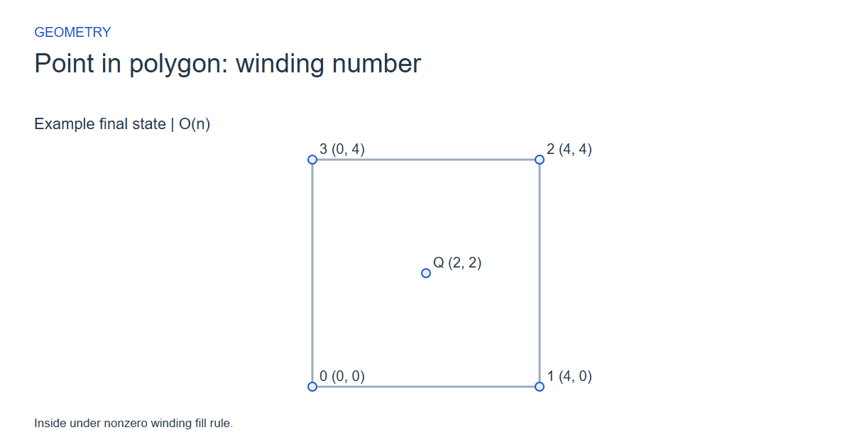
0,0;4,0;4,4;0,4|2,2These checkpoints follow the actual example timeline. State details show the stored values and decisions; use the visualization to inspect every intervening step.
Step 0: Exact integer predicates; equal scale on both coordinate axes.
State at this checkpoint
{
  "values": [
    0,
    1,
    2,
    3,
    4
  ],
  "active": [],
  "kind": "graph",
  "points": [
    [
      0,
      0
    ],
    [
      4,
      0
    ],
    [
      4,
      4
    ],
    [
      0,
      4
    ],
    [
      2,
      2
    ]
  ],
  "nodeLabels": [
    "0 (0, 0)",
    "1 (4, 0)",
    "2 (4, 4)",
    "3 (0, 4)",
    "Q (2, 2)"
  ],
  "directed": false,
  "chosen": [],
  "visited": [],
  "result": 0,
  "output": []
}
Step 1: Edge 0: cross product 8; signed winding 0.
State at this checkpoint
{
  "values": [
    0,
    1,
    2,
    3,
    4
  ],
  "active": [
    0,
    1,
    4
  ],
  "kind": "graph",
  "points": [
    [
      0,
      0
    ],
    [
      4,
      0
    ],
    [
      4,
      4
    ],
    [
      0,
      4
    ],
    [
      2,
      2
    ]
  ],
  "nodeLabels": [
    "0 (0, 0)",
    "1 (4, 0)",
    "2 (4, 4)",
    "3 (0, 4)",
    "Q (2, 2)"
  ],
  "directed": false,
  "chosen": [
    0
  ],
  "visited": [],
  "result": 0,
  "output": []
}
Step 3: Edge 2: cross product 8; signed winding 1.
State at this checkpoint
{
  "values": [
    0,
    1,
    2,
    3,
    4
  ],
  "active": [
    2,
    3,
    4
  ],
  "kind": "graph",
  "points": [
    [
      0,
      0
    ],
    [
      4,
      0
    ],
    [
      4,
      4
    ],
    [
      0,
      4
    ],
    [
      2,
      2
    ]
  ],
  "nodeLabels": [
    "0 (0, 0)",
    "1 (4, 0)",
    "2 (4, 4)",
    "3 (0, 4)",
    "Q (2, 2)"
  ],
  "directed": false,
  "chosen": [
    2
  ],
  "visited": [],
  "result": 0,
  "output": []
}
Step 4: Edge 3: cross product 8; signed winding 1.
State at this checkpoint
{
  "values": [
    0,
    1,
    2,
    3,
    4
  ],
  "active": [
    3,
    0,
    4
  ],
  "kind": "graph",
  "points": [
    [
      0,
      0
    ],
    [
      4,
      0
    ],
    [
      4,
      4
    ],
    [
      0,
      4
    ],
    [
      2,
      2
    ]
  ],
  "nodeLabels": [
    "0 (0, 0)",
    "1 (4, 0)",
    "2 (4, 4)",
    "3 (0, 4)",
    "Q (2, 2)"
  ],
  "directed": false,
  "chosen": [
    3
  ],
  "visited": [],
  "result": 0,
  "output": []
}
Step 5: Inside under nonzero winding fill rule.
State at this checkpoint
{
  "values": [
    0,
    1,
    2,
    3,
    4
  ],
  "active": [
    4
  ],
  "kind": "graph",
  "points": [
    [
      0,
      0
    ],
    [
      4,
      0
    ],
    [
      4,
      4
    ],
    [
      0,
      4
    ],
    [
      2,
      2
    ]
  ],
  "nodeLabels": [
    "0 (0, 0)",
    "1 (4, 0)",
    "2 (4, 4)",
    "3 (0, 4)",
    "Q (2, 2)"
  ],
  "directed": false,
  "chosen": [],
  "visited": [],
  "result": 1,
  "output": []
}
Expected final state
Inside under nonzero winding fill rule.
Complexity and input bounds
Family: Geometry. Time complexity: O(n).
Implementation detail: Up to twelve vertices, query and coordinates -20..20. Return 2 boundary, 1 nonzero-winding interior, 0 outside. Empty native path is outside. All orientation calculations use exact bounded integers. Both views preserve the coordinate aspect ratio. Independent fixtures cover degeneracies and deterministic outcomes in all nine languages.
Space complexity: O(n) index storage for closest-pair sweep; O(1) predicate state otherwise, excluding inputs and saved frames.
Working-space bounds describe algorithm state and any explicitly noted output, excluding the visualization's saved timeline. Recording frames can use more memory than running the function alone. Here n is sequence length, V and E are vertex and edge counts, and other parameters refer to the named input dimensions.
Polygon vertices x,y separated by ;, then |queryX,queryY. 3..12 vertices; integers -20..20. Boundary=2, inside=1, outside=0.
The playground validates these limits before starting. Downloaded functions are callable implementations, with parameter and output-buffer contracts in their comments; they do not all repeat the playground's input validation.
Common mistakes and limitations
Use half-open vertical intervals and strict orientation signs. Handle repeated and horizontal edges, and avoid treating complex paths as simple polygons without specifying a rule.
Further reading
For background on algorithm analysis and the JavaScript function interface:
- MIT OpenCourseWare: algorithm design and analysis foundations
- MDN: JavaScript function parameters and return values
Editorial and testing approach · Browse all algorithm guides
Complete JavaScript implementation
1 2 3 4 5 6 7 8 | // Closed polygon path n 0..12; x/y/query integer -20..20. Return 2 on boundary, otherwise 1 inside under nonzero signed winding rule, or 0 outside. Empty path returns 0. Repeated vertices and self-intersections are supported under the stated fill rule, which may differ between algorithms. Half-open vertical crossings avoid vertex double counting; exact integer orientation avoids division. O(n) time, O(1) auxiliary space. Reference snippets assume validated playground inputs. Fixed scratch buffers have 256 slots. Sorting variants may use a different traversal strategy than the animation. function algorithm(x, y, n, qx, qy) { let count = 0; let next = 0; let turn = 0; for (let i = 0; i < n; i++) { next = (i+1)%n; turn = (x[next]-x[i])*(qy-y[i])-(y[next]-y[i])*(qx-x[i]); if (turn == 0 && (qx-x[i])*(qx-x[next]) <= 0 && (qy-y[i])*(qy-y[next]) <= 0) { return 2; } if (y[i] <= qy && y[next] > qy && turn > 0) { count++; } if (y[i] > qy && y[next] <= qy && turn < 0) { count--; } } if (count != 0) { return 1; } return 0; } |
Source
Original-author technical reference comparing polygon containment strategies, not an asserted first-invention paper.
- Point in Polygon Strategies
Eric Haines (1994). Author reference.