Published by Dimitris Kougioumtzis · Updated
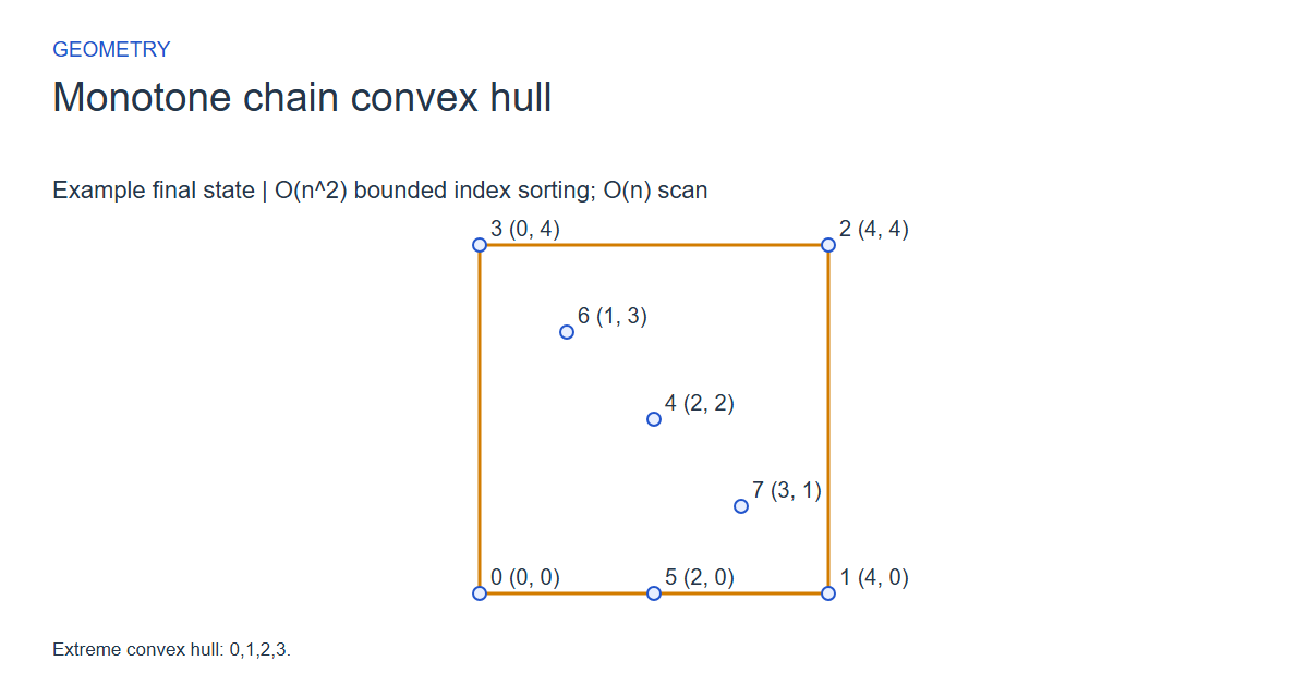
Build the extreme convex boundary while omitting interior collinear points. Actual coordinates use the same scale on both axes.
Sort points lexicographically and build lower and upper chains, removing non-left turns.
When to use Monotone chain convex hull
Finding the extreme convex boundary of a planar point set for shape analysis and geometric preprocessing.
Choosing an alternative
Two directional scans avoid angular sorting and join at the extreme endpoints.
Worked example: input and state changes
Example input
0,0;4,0;4,4;0,4;2,2;2,0;1,3;3,1These checkpoints follow the actual example timeline. State details show the stored values and decisions; use the visualization to inspect every intervening step.
Step 0: Coincident points use the first input index. Coordinate axes have equal scale.
State at this checkpoint
{
  "values": [
    0,
    1,
    2,
    3,
    4,
    5,
    6,
    7
  ],
  "active": [],
  "kind": "graph",
  "points": [
    [
      0,
      0
    ],
    [
      4,
      0
    ],
    [
      4,
      4
    ],
    [
      0,
      4
    ],
    [
      2,
      2
    ],
    [
      2,
      0
    ],
    [
      1,
      3
    ],
    [
      3,
      1
    ]
  ],
  "nodeLabels": [
    "0 (0, 0)",
    "1 (4, 0)",
    "2 (4, 4)",
    "3 (0, 4)",
    "4 (2, 2)",
    "5 (2, 0)",
    "6 (1, 3)",
    "7 (3, 1)"
  ],
  "directed": false,
  "chosen": [],
  "visited": [],
  "result": 0,
  "output": []
}
Step 7: Extend lower chain.
State at this checkpoint
{
  "values": [
    0,
    1,
    2,
    3,
    4,
    5,
    6,
    7
  ],
  "active": [
    4
  ],
  "kind": "graph",
  "points": [
    [
      0,
      0
    ],
    [
      4,
      0
    ],
    [
      4,
      4
    ],
    [
      0,
      4
    ],
    [
      2,
      2
    ],
    [
      2,
      0
    ],
    [
      1,
      3
    ],
    [
      3,
      1
    ]
  ],
  "nodeLabels": [
    "0 (0, 0)",
    "1 (4, 0)",
    "2 (4, 4)",
    "3 (0, 4)",
    "4 (2, 2)",
    "5 (2, 0)",
    "6 (1, 3)",
    "7 (3, 1)"
  ],
  "directed": false,
  "chosen": [
    0,
    1
  ],
  "visited": [
    0,
    5,
    4
  ],
  "result": 0,
  "output": []
}
Step 14: Extend upper chain.
State at this checkpoint
{
  "values": [
    0,
    1,
    2,
    3,
    4,
    5,
    6,
    7
  ],
  "active": [
    2
  ],
  "kind": "graph",
  "points": [
    [
      0,
      0
    ],
    [
      4,
      0
    ],
    [
      4,
      4
    ],
    [
      0,
      4
    ],
    [
      2,
      2
    ],
    [
      2,
      0
    ],
    [
      1,
      3
    ],
    [
      3,
      1
    ]
  ],
  "nodeLabels": [
    "0 (0, 0)",
    "1 (4, 0)",
    "2 (4, 4)",
    "3 (0, 4)",
    "4 (2, 2)",
    "5 (2, 0)",
    "6 (1, 3)",
    "7 (3, 1)"
  ],
  "directed": false,
  "chosen": [],
  "visited": [
    2
  ],
  "result": 0,
  "output": []
}
Step 20: Extend upper chain.
State at this checkpoint
{
  "values": [
    0,
    1,
    2,
    3,
    4,
    5,
    6,
    7
  ],
  "active": [
    5
  ],
  "kind": "graph",
  "points": [
    [
      0,
      0
    ],
    [
      4,
      0
    ],
    [
      4,
      4
    ],
    [
      0,
      4
    ],
    [
      2,
      2
    ],
    [
      2,
      0
    ],
    [
      1,
      3
    ],
    [
      3,
      1
    ]
  ],
  "nodeLabels": [
    "0 (0, 0)",
    "1 (4, 0)",
    "2 (4, 4)",
    "3 (0, 4)",
    "4 (2, 2)",
    "5 (2, 0)",
    "6 (1, 3)",
    "7 (3, 1)"
  ],
  "directed": false,
  "chosen": [
    0,
    1
  ],
  "visited": [
    2,
    4,
    5
  ],
  "result": 0,
  "output": []
}
Step 27: Extreme convex hull: 0,1,2,3.
State at this checkpoint
{
  "values": [
    0,
    1,
    2,
    3,
    4,
    5,
    6,
    7
  ],
  "active": [],
  "kind": "graph",
  "points": [
    [
      0,
      0
    ],
    [
      4,
      0
    ],
    [
      4,
      4
    ],
    [
      0,
      4
    ],
    [
      2,
      2
    ],
    [
      2,
      0
    ],
    [
      1,
      3
    ],
    [
      3,
      1
    ]
  ],
  "nodeLabels": [
    "0 (0, 0)",
    "1 (4, 0)",
    "2 (4, 4)",
    "3 (0, 4)",
    "4 (2, 2)",
    "5 (2, 0)",
    "6 (1, 3)",
    "7 (3, 1)"
  ],
  "directed": false,
  "chosen": [
    0,
    1,
    2,
    3
  ],
  "visited": [
    0,
    1,
    2,
    3
  ],
  "result": 4,
  "output": [
    0,
    1,
    2,
    3
  ]
}
Expected final state
Extreme convex hull: 0,1,2,3.
Complexity and input bounds
Family: Geometry. Time complexity: O(n^2) bounded index sorting; O(n) scan.
Implementation detail: Coordinates are integers -20..20, with at most twelve input points. Downloads accept separate x and y arrays and return the hull count while writing original point indices counterclockwise from the lexicographic minimum. Empty native input returns zero. Both displays preserve equal coordinate scale. Independent supporting-line fixtures verify extrema, duplicates and degenerate inputs in all nine languages.
Space complexity: O(n) working point and hull storage, plus recorded visualization frames.
Working-space bounds describe algorithm state and any explicitly noted output, excluding the visualization's saved timeline. Recording frames can use more memory than running the function alone. Here n is sequence length, V and E are vertex and edge counts, and other parameters refer to the named input dimensions.
1..12 points x,y separated by ;, integer coordinates -20..20. Coincident points use their first input index; output is CCW from the lexicographic minimum.
The playground validates these limits before starting. Downloaded functions are callable implementations, with parameter and output-buffer contracts in their comments; they do not all repeat the playground's input validation.
Common mistakes and limitations
Retain the first index for coincident points. Exclude interior collinear points, handle a single unique point and all-collinear sets, and canonicalize orientation before comparing hulls.
Further reading
For background on algorithm analysis and the JavaScript function interface:
- MIT OpenCourseWare: algorithm design and analysis foundations
- MDN: JavaScript function parameters and return values
Editorial and testing approach · Browse all algorithm guides
Complete JavaScript implementation
1 2 3 4 5 6 7 8 9 10 11 12 13 14 15 16 17 18 19 | // Planar convex hull, n 0..12 integer x/y coordinates -20..20, output capacity n. Returns number of extreme hull vertices and writes original input indices counterclockwise from lexicographically smallest coordinate. Coincident points use first input index; interior collinear boundary points are omitted. Collinear input returns its two endpoints, one unique point returns one, empty returns zero. Coordinates are unchanged; all orientation/distance tests use exact bounded integer arithmetic. Portable versions use O(n^2) stable index preprocessing (and angular insertion sorting for Graham); monotone/Graham scans are O(n), Jarvis wrapping O(n*h), Quickhull worst case O(n^2). Fixed O(n) scratch/explicit stacks; Python uses its standard index sort and recursive Quickhull. Reference snippets assume validated playground inputs. Fixed scratch buffers have 256 slots. Sorting variants may use a different traversal strategy than the animation. function algorithm(x, y, n, output) { if (n == 0) { return 0; } let order = Array(256).fill(0); let points = Array(256).fill(0); let hull = Array(256).fill(0); let key = 0; let cursor = 0; let count = 0; let id = 0; let size = 0; for (let i = 0; i < n; i++) { order[i] = i; } for (let i = 1; i < n; i++) { key = order[i]; cursor = i-1; while (cursor >= 0 && (x[order[cursor]] > x[key] || (x[order[cursor]] == x[key] && y[order[cursor]] > y[key]))) { order[cursor+1] = order[cursor]; cursor--; } order[cursor+1] = key; } for (let i = 0; i < n; i++) { id = order[i]; if (count == 0 || x[id] != x[points[count-1]] || y[id] != y[points[count-1]]) { points[count] = id; count++; } } if (count == 1) { output[0] = points[0]; return 1; } for (let i = 0; i < count; i++) { while (size >= 2 && ((x[hull[size-1]]-x[hull[size-2]])*(y[points[i]]-y[hull[size-2]])-(y[hull[size-1]]-y[hull[size-2]])*(x[points[i]]-x[hull[size-2]])) <= 0) { size--; } hull[size] = points[i]; size++; } let threshold = size+1; for (let i = count-2; i >= 0; i--) { while (size >= threshold && ((x[hull[size-1]]-x[hull[size-2]])*(y[points[i]]-y[hull[size-2]])-(y[hull[size-1]]-y[hull[size-2]])*(x[points[i]]-x[hull[size-2]])) <= 0) { size--; } hull[size] = points[i]; size++; } size--; let area = 0; let best = 0; let nextIndex = 0; let swapValue = 0; let left = 0; let right = 0; for (let i = 0; i < size; i++) { nextIndex = (i+1)%size; area += x[hull[i]]*y[hull[nextIndex]]-y[hull[i]]*x[hull[nextIndex]]; } if (area < 0) { left = 0; right = size-1; while (left < right) { swapValue = hull[left]; hull[left] = hull[right]; hull[right] = swapValue; left++; right--; } } for (let i = 1; i < size; i++) { if (x[hull[i]] < x[hull[best]] || (x[hull[i]] == x[hull[best]] && y[hull[i]] < y[hull[best]])) { best = i; } } for (let i = 0; i < size; i++) { output[i] = hull[(best+i)%size]; } return size; } |
Source
Primary research for the named hull method. This bounded teaching implementation uses insertion-based preprocessing, so its stated complexity includes quadratic sorting rather than claiming an optimal library sort.
- Another efficient algorithm for convex hulls in two dimensions
A.M. Andrew (1979). Research paper.