Published by Dimitris Kougioumtzis · Updated
Sort by finish time, then choose compatible jobs with maximum total value. Reconstruct the selected original job indices.
Sort by finish time, then compare skipping a job with taking it plus the best compatible prefix.
When to use Weighted interval scheduling
Scheduling compatible activities with unequal rewards.
Choosing an alternative
Earliest-finish activity selection maximizes count rather than value.
Worked example: input and state changes
Example input
1,3,5;2,5,6;4,6,5;6,7,4These checkpoints follow the actual example timeline. State details show the stored values and decisions; use the visualization to inspect every intervening step.
Step 0: Initial state.
State at this checkpoint
{
  "values": [
    0,
    0,
    0,
    0,
    0
  ],
  "active": []
}
Step 1: Job 0: take value 5 plus compatible prefix, or skip; best 5.
State at this checkpoint
{
  "values": [
    0,
    5,
    0,
    0,
    0
  ],
  "active": [
    1
  ],
  "jobs": [
    {
      "data": [
        1,
        3,
        5
      ],
      "id": 0
    },
    {
      "data": [
        2,
        5,
        6
      ],
      "id": 1
    },
    {
      "data": [
        4,
        6,
        5
      ],
      "id": 2
    },
    {
      "data": [
        6,
        7,
        4
      ],
      "id": 3
    }
  ]
}
Step 3: Job 2: take value 5 plus compatible prefix, or skip; best 10.
State at this checkpoint
{
  "values": [
    0,
    5,
    6,
    10,
    0
  ],
  "active": [
    3
  ],
  "jobs": [
    {
      "data": [
        1,
        3,
        5
      ],
      "id": 0
    },
    {
      "data": [
        2,
        5,
        6
      ],
      "id": 1
    },
    {
      "data": [
        4,
        6,
        5
      ],
      "id": 2
    },
    {
      "data": [
        6,
        7,
        4
      ],
      "id": 3
    }
  ]
}
Step 4: Job 3: take value 4 plus compatible prefix, or skip; best 14.
State at this checkpoint
{
  "values": [
    0,
    5,
    6,
    10,
    14
  ],
  "active": [
    4
  ],
  "jobs": [
    {
      "data": [
        1,
        3,
        5
      ],
      "id": 0
    },
    {
      "data": [
        2,
        5,
        6
      ],
      "id": 1
    },
    {
      "data": [
        4,
        6,
        5
      ],
      "id": 2
    },
    {
      "data": [
        6,
        7,
        4
      ],
      "id": 3
    }
  ]
}
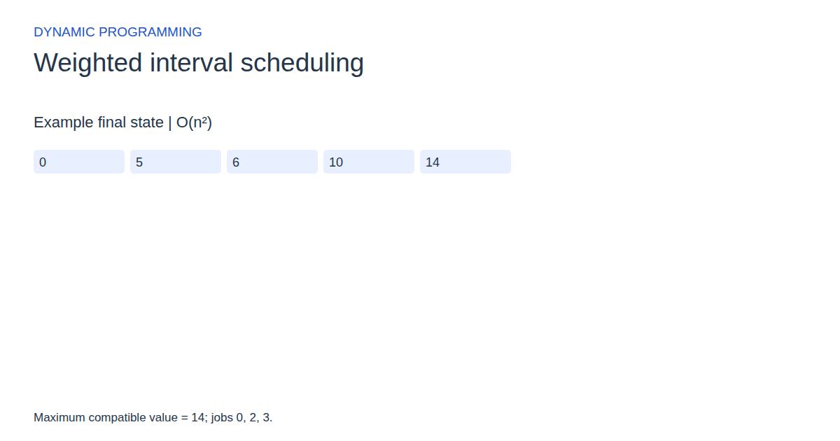
Step 5: Maximum compatible value = 14; jobs 0, 2, 3.
State at this checkpoint
{
  "values": [
    0,
    5,
    6,
    10,
    14
  ],
  "active": [],
  "jobs": [
    {
      "data": [
        1,
        3,
        5
      ],
      "id": 0
    },
    {
      "data": [
        2,
        5,
        6
      ],
      "id": 1
    },
    {
      "data": [
        4,
        6,
        5
      ],
      "id": 2
    },
    {
      "data": [
        6,
        7,
        4
      ],
      "id": 3
    }
  ],
  "result": 14,
  "jobsSelected": [
    0,
    2,
    3
  ]
}
Expected final state
Maximum compatible value = 14; jobs 0, 2, 3.
Complexity and input bounds
Family: Dynamic programming. Time complexity: O(n²).
Space complexity: O(n) optimum and reconstruction arrays.
Working-space bounds describe algorithm state and any explicitly noted output, excluding the visualization's saved timeline. Recording frames can use more memory than running the function alone. Here n is sequence length, V and E are vertex and edge counts, and other parameters refer to the named input dimensions.
1–12 start,end,value triples separated by semicolons; 0 ≤ start < end ≤ 99 and value 0–99.
The playground validates these limits before starting. Downloaded functions are callable implementations, with parameter and output-buffer contracts in their comments; they do not all repeat the playground's input validation.
Common mistakes and limitations
This reference scans for compatibility; do not claim a binary-search predecessor bound for it.
Further reading
For background on algorithm analysis and the JavaScript function interface:
- MIT OpenCourseWare: algorithm design and analysis foundations
- MDN: JavaScript function parameters and return values
Editorial and testing approach · Browse all algorithm guides
Complete JavaScript implementation
1 2 3 4 5 6 7 8 9 10 11 12 13 14 15 16 17 18 | // 1–12 jobs with 0 ≤ start < end ≤ 99 and nonnegative values ≤ 99. Returns best value. output[0] is selected count; remaining entries are original indices in chronological order. Reference snippets assume validated playground inputs. Fixed scratch buffers have 256 slots. Sorting variants may use a different traversal strategy than the animation. function algorithm(starts, ends, values, n, output) { let order = Array(256).fill(0); let previous = Array(256).fill(0); let dp = Array(256).fill(0); for (let i = 0; i < n; i++) { order[i] = i; } for (let i = 1; i < n; i++) { let j = i; while (j > 0 && ends[order[j - 1]] > ends[order[j]]) { let t = order[j]; order[j] = order[j - 1]; order[j - 1] = t; j--; } } for (let i = 0; i < n; i++) { let k = order[i]; previous[i] = -1; for (let j = i - 1; j >= 0; j--) { if (ends[order[j]] <= starts[k]) { previous[i] = j; break; } } dp[i + 1] = dp[i]; let candidate = values[k] + dp[previous[i] + 1]; if (candidate > dp[i + 1]) { dp[i + 1] = candidate; } } let selected = Array(256).fill(0); let size = 0; let index = n - 1; while (index >= 0) { if (values[order[index]] + dp[previous[index] + 1] > dp[index]) { selected[size++] = order[index]; index = previous[index]; } else { index--; } } output[0] = size; for (let i = 0; i < size; i++) { output[i + 1] = selected[size - 1 - i]; } return dp[n]; } |
Source
Foundational dynamic-programming paper. It establishes the general method, not the first publication or exact recurrence of this particular teaching example.
- The theory of dynamic programming
Richard Bellman (1954). Foundational method paper.