Published by Dimitris Kougioumtzis · Updated
Track discovery times, low links and an active stack; pop one strongly connected component at each root.
Track discovery times, low links, and an active stack; an SCC root pops one complete component from that stack.
When to use Tarjan strongly connected components
Collapsing directed cycles into a condensation graph.
Choosing an alternative
Kosaraju uses a second traversal on reversed edges.
Worked example: input and state changes
Example input
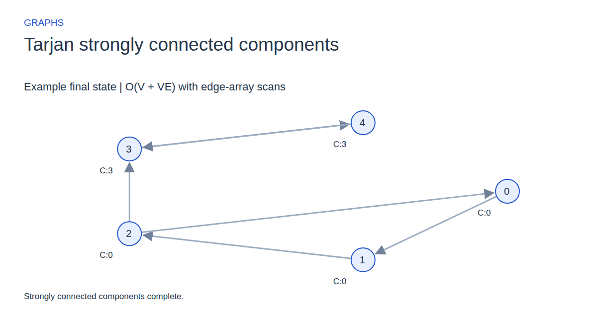
0,1,1;1,2,1;2,0,1;2,3,1;3,4,1;4,3,1These checkpoints follow the actual example timeline. State details show the stored values and decisions; use the visualization to inspect every intervening step.
Step 0: Initialize graph state.
State at this checkpoint
{
  "values": [
    "-",
    "-",
    "-",
    "-",
    "-"
  ],
  "active": [],
  "kind": "graph",
  "chosen": [],
  "visited": []
}
Step 4: Inspect 2 > 0; low[2]=0.
State at this checkpoint
{
  "values": [
    "d:0 l:0",
    "d:1 l:1",
    "d:2 l:0",
    "d:-1 l:-1",
    "d:-1 l:-1"
  ],
  "active": [
    2,
    0
  ],
  "kind": "graph",
  "chosen": [],
  "visited": [],
  "discovery": [
    0,
    1,
    2,
    -1,
    -1
  ],
  "low": [
    0,
    1,
    0,
    -1,
    -1
  ],
  "components": [
    -1,
    -1,
    -1,
    -1,
    -1
  ],
  "stack": [
    0,
    1,
    2
  ],
  "finish": []
}
Step 8: Inspect 3 > 4; low[3]=3.
State at this checkpoint
{
  "values": [
    "d:0 l:0",
    "d:1 l:1",
    "d:2 l:0",
    "d:3 l:3",
    "d:4 l:3"
  ],
  "active": [
    3,
    4
  ],
  "kind": "graph",
  "chosen": [],
  "visited": [],
  "discovery": [
    0,
    1,
    2,
    3,
    4
  ],
  "low": [
    0,
    1,
    0,
    3,
    3
  ],
  "components": [
    -1,
    -1,
    -1,
    -1,
    -1
  ],
  "stack": [
    0,
    1,
    2,
    3,
    4
  ],
  "finish": [
    4
  ]
}
Step 11: Inspect 1 > 2; low[1]=0.
State at this checkpoint
{
  "values": [
    "d:0 l:0",
    "d:1 l:0",
    "d:2 l:0",
    "C:3",
    "C:3"
  ],
  "active": [
    1,
    2
  ],
  "kind": "graph",
  "chosen": [],
  "visited": [],
  "discovery": [
    0,
    1,
    2,
    3,
    4
  ],
  "low": [
    0,
    0,
    0,
    3,
    3
  ],
  "components": [
    -1,
    -1,
    -1,
    3,
    3
  ],
  "stack": [
    0,
    1,
    2
  ],
  "finish": [
    4,
    3,
    2
  ]
}
Step 15: Strongly connected components complete.
State at this checkpoint
{
  "values": [
    "C:0",
    "C:0",
    "C:0",
    "C:3",
    "C:3"
  ],
  "active": [],
  "kind": "graph",
  "chosen": [],
  "visited": [
    0,
    1,
    2,
    3,
    4
  ],
  "result": 2,
  "components": [
    0,
    0,
    0,
    3,
    3
  ]
}
Expected final state
Strongly connected components complete.
Complexity and input bounds
Family: Graphs. Time complexity: O(V + VE) with edge-array scans.
Space complexity: O(V) discovery, DFS, and active-stack state.
Working-space bounds describe algorithm state and any explicitly noted output, excluding the visualization's saved timeline. Recording frames can use more memory than running the function alone. Here n is sequence length, V and E are vertex and edge counts, and other parameters refer to the named input dimensions.
Directed edges as source,target,weight; separated by semicolons. Nodes 0–7, positive weights 1–99. Start node is 0. At most 16 edges. Weights are ignored. Vertices include every index from 0 to the highest endpoint.
The playground validates these limits before starting. Downloaded functions are callable implementations, with parameter and output-buffer contracts in their comments; they do not all repeat the playground's input validation.
Common mistakes and limitations
Only edges to still-active vertices affect the relevant back-edge low link; completed SCCs must remain separate.
Further reading
For background on algorithm analysis and the JavaScript function interface:
- MIT OpenCourseWare: algorithm design and analysis foundations
- MDN: JavaScript function parameters and return values
Editorial and testing approach · Browse all algorithm guides
Complete JavaScript implementation
1 2 3 4 5 6 7 8 9 10 11 12 13 14 15 16 17 18 19 20 21 22 23 24 25 26 27 28 29 30 | // Edge arrays from/to/weight; 1..8 vertices indexed 0..vertices-1, 0..16 edges, endpoints in bounds. Weights ignored. Output buffer at least 256 integers. Directed SCCs: returns component count; output[v] is the smallest vertex in v's component. Reference snippets assume validated playground inputs. Fixed scratch buffers have 256 slots. Sorting variants may use a different traversal strategy than the animation. function algorithm(from, to, weight, edges, vertices, output) { let disc = Array(256).fill(0); let low = Array(256).fill(0); let active = Array(256).fill(0); let parent = Array(256).fill(0); let cursor = Array(256).fill(0); let dfs = Array(256).fill(0); let stack = Array(256).fill(0); let group = Array(256).fill(0); let root = 0; let u = 0; let v = 0; let index = 0; let top = 0; let size = 0; let clock = 0; let count = 0; let length = 0; let label = 0; for (u = 0; u < vertices; u++) { disc[u] = -1; parent[u] = -1; output[u] = -1; } for (root = 0; root < vertices; root++) { if (disc[root] >= 0) { continue; } disc[root] = clock; low[root] = clock++; active[root] = 1; stack[size++] = root; dfs[top++] = root; while (top > 0) { u = dfs[top - 1]; index = cursor[u]; while (index < edges && from[index] != u) { index++; } cursor[u] = index + 1; if (index < edges) { v = to[index]; if (disc[v] < 0) { parent[v] = u; disc[v] = clock; low[v] = clock++; active[v] = 1; stack[size++] = v; dfs[top++] = v; } else if (active[v] != 0 && disc[v] < low[u]) { low[u] = disc[v]; } } else { top--; if (low[u] == disc[u]) { length = 0; label = u; do { v = stack[--size]; active[v] = 0; group[length++] = v; if (v < label) { label = v; } } while (v != u); for (index = 0; index < length; index++) { output[group[index]] = label; } count++; } v = parent[u]; if (v >= 0 && low[u] < low[v]) { low[v] = low[u]; } } } } return count; } |
Source
Primary research source for the algorithm or its underlying method. The playground is a bounded teaching implementation, not the publication's original program.
- Depth-First Search and Linear Graph Algorithms
Robert Tarjan (1972). Research paper.