Published by Dimitris Kougioumtzis · Updated
Minimize total cost from top-left to bottom-right, including both endpoints; move only right or down.
Add each cell's weight to the cheaper reachable cost from above or left, exploiting the movement graph's acyclicity.
When to use Minimum-cost monotone grid path
Weighted monotone route planning.
Choosing an alternative
A* allows obstacles and four-direction movement.
Worked example: input and state changes
Example input
1,3,1;1,5,1;4,2,1These checkpoints follow the actual example timeline. State details show the stored values and decisions; use the visualization to inspect every intervening step.
Step 0: Minimum-cost table begins empty.
State at this checkpoint
{
  "values": [
    0,
    0,
    0,
    0,
    0,
    0,
    0,
    0,
    0
  ],
  "active": [],
  "kind": "matrix",
  "columns": 3,
  "costs": [
    1,
    3,
    1,
    1,
    5,
    1,
    4,
    2,
    1
  ]
}
Step 3: Cell [0,2]: total cost 5.
State at this checkpoint
{
  "values": [
    1,
    4,
    5,
    0,
    0,
    0,
    0,
    0,
    0
  ],
  "active": [
    2
  ],
  "kind": "matrix",
  "columns": 3,
  "costs": [
    1,
    3,
    1,
    1,
    5,
    1,
    4,
    2,
    1
  ]
}
Step 5: Cell [1,1]: total cost 7.
State at this checkpoint
{
  "values": [
    1,
    4,
    5,
    2,
    7,
    0,
    0,
    0,
    0
  ],
  "active": [
    4
  ],
  "kind": "matrix",
  "columns": 3,
  "costs": [
    1,
    3,
    1,
    1,
    5,
    1,
    4,
    2,
    1
  ]
}
Step 8: Cell [2,1]: total cost 8.
State at this checkpoint
{
  "values": [
    1,
    4,
    5,
    2,
    7,
    6,
    6,
    8,
    0
  ],
  "active": [
    7
  ],
  "kind": "matrix",
  "columns": 3,
  "costs": [
    1,
    3,
    1,
    1,
    5,
    1,
    4,
    2,
    1
  ]
}
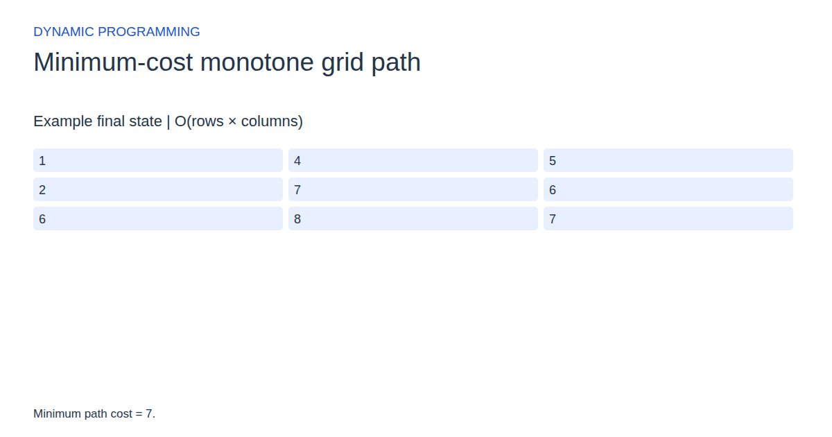
Step 10: Minimum path cost = 7.
State at this checkpoint
{
  "values": [
    1,
    4,
    5,
    2,
    7,
    6,
    6,
    8,
    7
  ],
  "active": [],
  "kind": "matrix",
  "columns": 3,
  "costs": [
    1,
    3,
    1,
    1,
    5,
    1,
    4,
    2,
    1
  ]
}
Expected final state
Minimum path cost = 7.
Complexity and input bounds
Family: Dynamic programming. Time complexity: O(rows × columns).
Space complexity: O(rows times columns) displayed table.
Working-space bounds describe algorithm state and any explicitly noted output, excluding the visualization's saved timeline. Recording frames can use more memory than running the function alone. Here n is sequence length, V and E are vertex and edge counts, and other parameters refer to the named input dimensions.
Up to 8 rows of 1–8 costs (0–99), separated by semicolons. All rows need the same number of columns.
The playground validates these limits before starting. Downloaded functions are callable implementations, with parameter and output-buffer contracts in their comments; they do not all repeat the playground's input validation.
Common mistakes and limitations
The start-cell weight is included, and diagonal or backward moves are not allowed.
Further reading
For background on algorithm analysis and the JavaScript function interface:
- MIT OpenCourseWare: algorithm design and analysis foundations
- MDN: JavaScript function parameters and return values
Editorial and testing approach · Browse all algorithm guides
Complete JavaScript implementation
1 2 3 4 5 6 7 8 9 10 11 12 13 14 | // Row-major costs from 0–99, each dimension 1–8. Returns minimum right/down path cost including both endpoints. Reference snippets assume validated playground inputs. Fixed scratch buffers have 256 slots. Sorting variants may use a different traversal strategy than the animation. function algorithm(costs, rows, columns) { let dp = Array(256).fill(0); for (let r = 0; r < rows; r++) { for (let c = 0; c < columns; c++) { let i = r * columns + c; let previous = 0; if (r == 0 && c > 0) { previous = dp[i - 1]; } else if (c == 0 && r > 0) { previous = dp[i - columns]; } else if (r > 0 && c > 0) { previous = dp[i - 1]; if (dp[i - columns] < previous) { previous = dp[i - columns]; } } dp[i] = costs[i] + previous; } } return dp[rows * columns - 1]; } |
Source
Foundational dynamic-programming paper. It establishes the general method, not the first publication or exact recurrence of this particular teaching example.
- The theory of dynamic programming
Richard Bellman (1954). Foundational method paper.