Published by Dimitris Kougioumtzis · Updated
Explore open cells depth first and undo dead-end path choices. Visited cells are retained to avoid repeating failed regions; the first path need not be shortest.
Treat each open grid cell as a vertex with orthogonal edges. Walk depth first, retaining visited marks and undoing only the current path when a dead end is reached. Stop on the first route to the goal.
When to use Depth-first maze solving
Teaching grid traversal, visited-state pruning and path reconstruction in a maze.
Choosing an alternative
Breadth-first search finds a shortest unweighted route. This DFS view finds the first route under a fixed neighbor order and may explore long detours.
Worked example: input and state changes
Example input
0,0,1,0;1,0,1,0;0,0,0,0These checkpoints follow the actual example timeline. State details show the stored values and decisions; use the visualization to inspect every intervening step.
Step 0: 0 open, 1 wall; visit neighbors up, right, down, left.
State at this checkpoint
{
  "values": [
    0,
    0,
    1,
    0,
    1,
    0,
    1,
    0,
    0,
    0,
    0,
    0
  ],
  "active": [],
  "kind": "matrix",
  "columns": 4,
  "result": 0,
  "output": [
    0
  ]
}
Step 2: Enter cell 1.
State at this checkpoint
{
  "values": [
    3,
    3,
    1,
    0,
    1,
    0,
    1,
    0,
    0,
    0,
    0,
    0
  ],
  "active": [
    1
  ],
  "kind": "matrix",
  "columns": 4,
  "result": 0,
  "output": [
    0
  ]
}
Step 4: Enter cell 9.
State at this checkpoint
{
  "values": [
    3,
    3,
    1,
    0,
    1,
    3,
    1,
    0,
    0,
    3,
    0,
    0
  ],
  "active": [
    9
  ],
  "kind": "matrix",
  "columns": 4,
  "result": 0,
  "output": [
    0
  ]
}
Step 5: Enter cell 10.
State at this checkpoint
{
  "values": [
    3,
    3,
    1,
    0,
    1,
    3,
    1,
    0,
    0,
    3,
    3,
    0
  ],
  "active": [
    10
  ],
  "kind": "matrix",
  "columns": 4,
  "result": 0,
  "output": [
    0
  ]
}
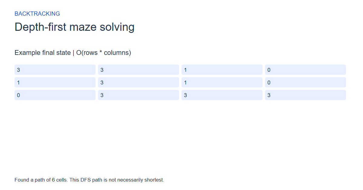
Step 7: Found a path of 6 cells. This DFS path is not necessarily shortest.
State at this checkpoint
{
  "values": [
    3,
    3,
    1,
    0,
    1,
    3,
    1,
    0,
    0,
    3,
    3,
    3
  ],
  "active": [],
  "kind": "matrix",
  "columns": 4,
  "result": 1,
  "output": [
    6,
    0,
    1,
    5,
    9,
    10,
    11
  ]
}
Expected final state
Found a path of 6 cells. This DFS path is not necessarily shortest.
Complexity and input bounds
Family: Backtracking. Time complexity: O(rows * columns).
Implementation detail: A binary grid has at most five rows and columns, top-left start and bottom-right goal. Neighbors are up, right, down, left. Playback uses 0 open, 1 wall, 2 explored and 3 current path. Downloads return a success flag and write path length followed by row-major indices.
Space complexity: O(rows times columns) visited state and DFS stack, plus output and recorded frames.
Working-space bounds describe algorithm state and any explicitly noted output, excluding the visualization's saved timeline. Recording frames can use more memory than running the function alone. Here n is sequence length, V and E are vertex and edge counts, and other parameters refer to the named input dimensions.
1..5 by 1..5 rectangular grid; rows separated by ;. 0 open, 1 wall. Start top-left; goal bottom-right. During playback 2 explored, 3 current path.
The playground validates these limits before starting. Downloaded functions are callable implementations, with parameter and output-buffer contracts in their comments; they do not all repeat the playground's input validation.
Common mistakes and limitations
Do not wrap a right or left step across row boundaries. Reject blocked endpoints. Keep explored marks after backtracking so failed regions are not traversed repeatedly.
Further reading
For background on algorithm analysis and the JavaScript function interface:
- MIT OpenCourseWare: algorithm design and analysis foundations
- MDN: JavaScript function parameters and return values
Editorial and testing approach · Browse all algorithm guides
Complete JavaScript implementation
1 2 3 4 5 6 7 8 9 | // Rectangular rows/cols 1..5, grid row-major 0 open/1 wall. Search from cell 0 to rows*cols-1 with neighbor order up, right, down, left. Returns 1 and writes [path length, then flattened cell indices] on success; returns 0 and writes length 0 on failure. Output capacity at least 1+rows*cols. Uses permanent visited marks and a DFS stack; not a shortest-path solver. O(rows*cols) time and scratch, no input mutation. Reference snippets assume validated playground inputs. Fixed scratch buffers have 256 slots. Sorting variants may use a different traversal strategy than the animation. function algorithm(grid, rows, cols, output) { output[0] = 0; let cells = rows*cols; if (grid[0] != 0 || grid[cells-1] != 0) { return 0; } let stack = Array(256).fill(0); let next = Array(256).fill(0); let seen = Array(256).fill(0); let depth = 0; let vertex = 0; let direction = 0; let candidate = 0; seen[0] = 1; while (depth >= 0) { vertex = stack[depth]; if (vertex == cells-1) { output[0] = depth+1; for (let i = 0; i <= depth; i++) { output[i+1] = stack[i]; } return 1; } if (next[depth] == 4) { depth--; } else { direction = next[depth]; next[depth]++; candidate = -1; if (direction == 0) { if (vertex >= cols) { candidate = vertex-cols; } } else { if (direction == 1) { if (vertex%cols+1 < cols) { candidate = vertex+1; } } else { if (direction == 2) { if (vertex+cols < cells) { candidate = vertex+cols; } } else { if (vertex%cols > 0) { candidate = vertex-1; } } } } if (candidate >= 0 && grid[candidate] == 0 && seen[candidate] == 0) { seen[candidate] = 1; depth++; stack[depth] = candidate; next[depth] = 0; } } } return 0; } |
Source
Primary research on depth-first graph methods, not a claim to the first maze-solving algorithm. The playground specializes ordinary DFS reachability and path reconstruction to a bounded grid.
- Depth-First Search and Linear Graph Algorithms
Robert Tarjan (1972). Research paper.