Published by Dimitris Kougioumtzis · Updated
Precompute power-of-two ancestors, equalize query depths, then lift both vertices until their parents coincide.
Store each vertex’s ancestor at distances 1, 2, 4 and so on. Lift the deeper query vertex to equal depth, then lift both vertices from large jumps to small until their immediate parents agree.
When to use Lowest common ancestor (binary lifting)
Answering common-ancestor queries in rooted hierarchies and computing tree distances from depths.
Choosing an alternative
Walking parent chains needs O(h) per query. Binary lifting uses O(n log n) preprocessing and O(log n) per query; Euler-tour RMQ is another approach.
Worked example: input and state changes
Example input
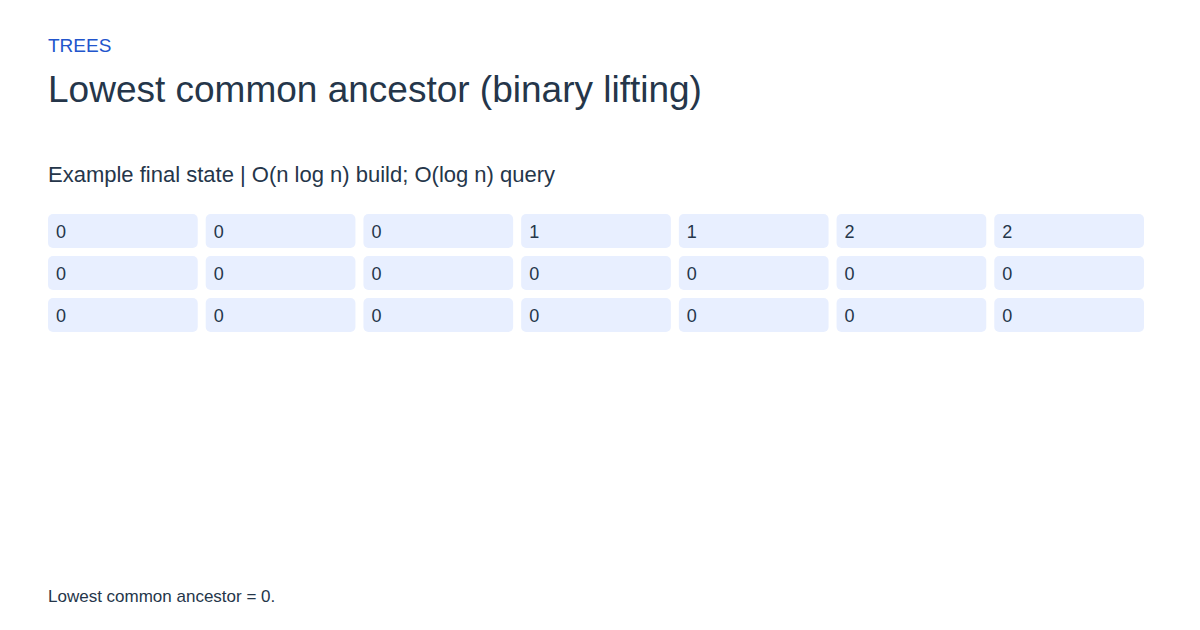
0,0,0,1,1,2,2 | 3,6These checkpoints follow the actual example timeline. State details show the stored values and decisions; use the visualization to inspect every intervening step.
Step 0: Row 0 stores parents (one-edge ancestors); root ancestors stay at root.
State at this checkpoint
{
  "values": [
    0,
    0,
    0,
    1,
    1,
    2,
    2,
    0,
    0,
    0,
    0,
    0,
    0,
    0,
    0,
    0,
    0,
    0,
    0,
    0,
    0
  ],
  "active": [],
  "kind": "matrix",
  "columns": 7,
  "depth": [
    0,
    1,
    1,
    2,
    2,
    2,
    2
  ],
  "u": 3,
  "v": 6
}
Step 4: Build ancestor 2^1 above vertex 3.
State at this checkpoint
{
  "values": [
    0,
    0,
    0,
    1,
    1,
    2,
    2,
    0,
    0,
    0,
    0,
    0,
    0,
    0,
    0,
    0,
    0,
    0,
    0,
    0,
    0
  ],
  "active": [
    10
  ],
  "kind": "matrix",
  "columns": 7,
  "depth": [
    0,
    1,
    1,
    2,
    2,
    2,
    2
  ],
  "u": 3,
  "v": 6
}
Step 8: Build ancestor 2^2 above vertex 0.
State at this checkpoint
{
  "values": [
    0,
    0,
    0,
    1,
    1,
    2,
    2,
    0,
    0,
    0,
    0,
    0,
    0,
    0,
    0,
    0,
    0,
    0,
    0,
    0,
    0
  ],
  "active": [
    14
  ],
  "kind": "matrix",
  "columns": 7,
  "depth": [
    0,
    1,
    1,
    2,
    2,
    2,
    2
  ],
  "u": 3,
  "v": 6
}
Step 12: Build ancestor 2^2 above vertex 4.
State at this checkpoint
{
  "values": [
    0,
    0,
    0,
    1,
    1,
    2,
    2,
    0,
    0,
    0,
    0,
    0,
    0,
    0,
    0,
    0,
    0,
    0,
    0,
    0,
    0
  ],
  "active": [
    18
  ],
  "kind": "matrix",
  "columns": 7,
  "depth": [
    0,
    1,
    1,
    2,
    2,
    2,
    2
  ],
  "u": 3,
  "v": 6
}
Step 16: Lowest common ancestor = 0.
State at this checkpoint
{
  "values": [
    0,
    0,
    0,
    1,
    1,
    2,
    2,
    0,
    0,
    0,
    0,
    0,
    0,
    0,
    0,
    0,
    0,
    0,
    0,
    0,
    0
  ],
  "active": [],
  "kind": "matrix",
  "columns": 7,
  "depth": [
    0,
    1,
    1,
    2,
    2,
    2,
    2
  ],
  "u": 0,
  "v": 2,
  "result": 0
}
Expected final state
Lowest common ancestor = 0.
Complexity and input bounds
Family: Trees. Time complexity: O(n log n) build; O(log n) query.
Implementation detail: The matrix rows show power-of-two ancestors; columns are vertices. The standalone function preprocesses the bounded tree for one query. Reusing the jump table is necessary to obtain the preprocessing benefit across many queries.
Space complexity: O(n log n) auxiliary space for the jump table, plus depths and saved visualization frames.
Working-space bounds describe algorithm state and any explicitly noted output, excluding the visualization's saved timeline. Recording frames can use more memory than running the function alone. Here n is sequence length, V and E are vertex and edge counts, and other parameters refer to the named input dimensions.
Parent list of 1..16 vertices | u,v. Vertex 0 is the root with parent 0; every other parent must have a smaller index.
The playground validates these limits before starting. Downloaded functions are callable implementations, with parameter and output-buffer contracts in their comments; they do not all repeat the playground's input validation.
Common mistakes and limitations
A vertex is its own ancestor. Root jumps must remain at the root. Parent arrays here use topological numbering: each non-root parent has a smaller index, which rules out cycles.
Further reading
For background on algorithm analysis and the JavaScript function interface:
- MIT OpenCourseWare: algorithm design and analysis foundations
- MDN: JavaScript function parameters and return values
Editorial and testing approach · Browse all algorithm guides
Complete JavaScript implementation
1 2 3 4 5 6 7 8 9 10 11 12 13 | // Rooted tree: 1..16 vertices, parent[0]=0, and 0 <= parent[i] < i for every i>0. Query u,v are valid vertex indices. Returns their lowest common ancestor; a vertex is its own ancestor. Builds a power-of-two ancestor table in O(n log n) time/space, then answers one query in O(log n). A reusable preprocessed table avoids rebuilding for repeated queries. Reference snippets assume validated playground inputs. Fixed scratch buffers have 256 slots. Sorting variants may use a different traversal strategy than the animation. function algorithm(parent, n, u, v) { let up = Array(256).fill(0); let depth = Array(256).fill(0); let levels = 1; let temp = 0; let difference = 0; while ((1 << levels) <= n) { levels++; } for (let i = 0; i < n; i++) { up[i] = parent[i]; if (i > 0) { depth[i] = depth[parent[i]] + 1; } } for (let k = 1; k < levels; k++) { for (let i = 0; i < n; i++) { up[k * n + i] = up[(k - 1) * n + up[(k - 1) * n + i]]; } } if (depth[u] < depth[v]) { temp = u; u = v; v = temp; } difference = depth[u] - depth[v]; for (let k = 0; k < levels; k++) { if ((difference & (1 << k)) != 0) { u = up[k * n + u]; } } if (u == v) { return u; } for (let k = levels - 1; k >= 0; k--) { if (up[k * n + u] != up[k * n + v]) { u = up[k * n + u]; v = up[k * n + v]; } } return parent[u]; } |
Source
Authored reference for the binary-lifting method, not an original research paper. No original publication for this exact depth-equalization variant has been verified here; the source explains power-of-two ancestor preprocessing and queries.
- Lowest Common Ancestor - Binary Lifting
CP-Algorithms contributors (2026). Authored algorithm reference (updated 2026).