Published by Dimitris Kougioumtzis · Updated
Search directed paths visiting every vertex exactly once and returning to the start. Weights are ignored; at most seven vertices.
Extend a directed path by an unvisited neighbor, undoing choices when a branch fails. Try starting vertices and successors in ascending order. A complete cycle must also have an edge from its last vertex to its start.
When to use Hamiltonian cycle backtracking
Studying exhaustive search, pruning, and small directed routing feasibility problems.
Choosing an alternative
Hierholzer consumes every edge; Hamiltonian search visits every vertex. Held-Karp uses subset dynamic programming for weighted tours.
Worked example: input and state changes
Example input
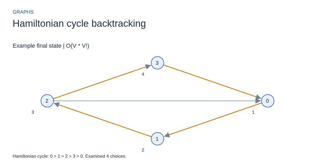
0,1,1;1,2,1;2,0,1;2,3,1;3,0,1These checkpoints follow the actual example timeline. State details show the stored values and decisions; use the visualization to inspect every intervening step.
Step 0: Try vertices in ascending order; undo a choice when no extension works.
State at this checkpoint
{
  "values": [
    "unvisited",
    "unvisited",
    "unvisited",
    "unvisited"
  ],
  "active": [],
  "kind": "graph",
  "chosen": [],
  "visited": [],
  "path": []
}
Step 1: Choose 0 at position 1.
State at this checkpoint
{
  "values": [
    1,
    "unvisited",
    "unvisited",
    "unvisited"
  ],
  "active": [
    0
  ],
  "kind": "graph",
  "chosen": [],
  "visited": [
    0
  ],
  "path": [
    0
  ]
}
Step 3: Choose 2 at position 3.
State at this checkpoint
{
  "values": [
    1,
    2,
    3,
    "unvisited"
  ],
  "active": [
    2
  ],
  "kind": "graph",
  "chosen": [
    0,
    1
  ],
  "visited": [
    0,
    1,
    2
  ],
  "path": [
    0,
    1,
    2
  ]
}
Step 4: Choose 3 at position 4.
State at this checkpoint
{
  "values": [
    1,
    2,
    3,
    4
  ],
  "active": [
    3
  ],
  "kind": "graph",
  "chosen": [
    0,
    1,
    3
  ],
  "visited": [
    0,
    1,
    2,
    3
  ],
  "path": [
    0,
    1,
    2,
    3
  ]
}
Step 5: Hamiltonian cycle: 0 > 1 > 2 > 3 > 0. Examined 4 choices.
State at this checkpoint
{
  "values": [
    1,
    2,
    3,
    4
  ],
  "active": [
    0
  ],
  "kind": "graph",
  "chosen": [
    0,
    1,
    3,
    4
  ],
  "visited": [
    0,
    1,
    2,
    3
  ],
  "path": [
    0,
    1,
    2,
    3,
    0
  ],
  "result": 5
}
Expected final state
Hamiltonian cycle: 0 > 1 > 2 > 3 > 0. Examined 4 choices.
Complexity and input bounds
Family: Graphs. Time complexity: O(V * V!).
Implementation detail: This is elementary exhaustive backtracking, not Rubin’s more elaborate deduction and edge-pruning procedure. The UI limits input to seven vertices and displays at most 500 intermediate snapshots, followed by the exact final result. Downloads return the number of output vertices or -1; cycle output repeats the start.
Space complexity: O(V^2) auxiliary space for the adjacency matrix plus O(V) search state; recorded visualization snapshots use additional space.
Working-space bounds describe algorithm state and any explicitly noted output, excluding the visualization's saved timeline. Recording frames can use more memory than running the function alone. Here n is sequence length, V and E are vertex and edge counts, and other parameters refer to the named input dimensions.
Directed edges as source,target,weight; separated by semicolons. Nodes 0–7, positive weights 1–99. Start node is 0. At most seven vertices; directed edges; weights ignored.
The playground validates these limits before starting. Downloaded functions are callable implementations, with parameter and output-buffer contracts in their comments; they do not all repeat the playground's input validation.
Common mistakes and limitations
An ordinary DFS traversal is not a Hamiltonian solution. Disconnected graphs may fail; parallel edges do not create new vertex orders. A self-loop is required for the one-vertex cycle used by this implementation.
Further reading
For background on algorithm analysis and the JavaScript function interface:
- MIT OpenCourseWare: algorithm design and analysis foundations
- MDN: JavaScript function parameters and return values
Editorial and testing approach · Browse all algorithm guides
Complete JavaScript implementation
1 2 3 4 5 6 7 8 9 10 11 12 13 14 15 16 17 18 19 20 21 22 23 24 25 26 | // Directed graph: 1..7 vertices, 0..16 edges, endpoints in range. Weights are ignored. Output capacity at least vertices+1. Returns the lexicographically first Hamiltonian cycle, including the repeated start, or -1 if none exists. A one-vertex path is valid; a one-vertex cycle requires a self-loop. Exhaustive backtracking takes O(V * V!) time and O(V^2) auxiliary space. Reference snippets assume validated playground inputs. Fixed scratch buffers have 256 slots. Sorting variants may use a different traversal strategy than the animation. function algorithm(from, to, weight, edges, vertices, output) { let adjacency = Array(256).fill(0); let path = Array(256).fill(0); let next = Array(256).fill(0); let used = Array(256).fill(0); let depth = 0; let v = 0; let valid = 0; for (let i = 0; i < edges; i++) { adjacency[from[i] * vertices + to[i]] = 1; } while (depth >= 0) { if (depth == vertices) { valid = adjacency[path[vertices - 1] * vertices + path[0]]; if (valid != 0) { for (let i = 0; i < vertices; i++) { output[i] = path[i]; } output[vertices] = path[0]; return vertices + 1; } depth--; used[path[depth]] = 0; continue; } v = next[depth]; while (v < vertices && (used[v] != 0 || (depth > 0 && adjacency[path[depth - 1] * vertices + v] == 0))) { v++; } if (v == vertices) { next[depth] = 0; depth--; if (depth >= 0) { used[path[depth]] = 0; } } else { next[depth] = v + 1; path[depth] = v; used[v] = 1; depth++; next[depth] = 0; } } return -1; } |
Source
Related primary research on Hamiltonian path and circuit search. The playground demonstrates elementary path-extension backtracking, without Rubin’s additional deductions; this citation is not a claim to reproduce that procedure.
- A Search Procedure for Hamilton Paths and Circuits
Frank Rubin (1974). Related research paper.