Published by Dimitris Kougioumtzis · Updated
Choose increasing input indices and prune branches with too few remaining positions.
Choose the next input index strictly after the previous one. Stop a branch when too few positions remain to complete k choices, and emit a row when the path reaches length k.
When to use Combinations by backtracking
Selecting fixed-size groups from a small labeled input sequence.
Choosing an alternative
Permutations distinguish different orders. Combinations preserve increasing input indices; equal values at different positions still represent different choices.
Worked example: input and state changes
Example input
1,2,3,4 | 2These checkpoints follow the actual example timeline. State details show the stored values and decisions; use the visualization to inspect every intervening step.
Step 0: Input 1,2,3,4. Build a choice path; completed rows appear below it.
State at this checkpoint
{
  "values": [
    "�",
    "�"
  ],
  "active": [],
  "kind": "matrix",
  "columns": 2,
  "result": 0,
  "output": []
}
Step 6: Emit result 2.
State at this checkpoint
{
  "values": [
    1,
    3,
    1,
    2,
    1,
    3
  ],
  "active": [],
  "kind": "matrix",
  "columns": 2,
  "result": 2,
  "output": [
    1,
    2,
    1,
    3
  ]
}
Step 13: Choose input index 2.
State at this checkpoint
{
  "values": [
    2,
    3,
    1,
    2,
    1,
    3,
    1,
    4
  ],
  "active": [],
  "kind": "matrix",
  "columns": 2,
  "result": 3,
  "output": [
    1,
    2,
    1,
    3,
    1,
    4
  ]
}
Step 19: Undo the choice and explore another branch.
State at this checkpoint
{
  "values": [
    "�",
    "�",
    1,
    2,
    1,
    3,
    1,
    4,
    2,
    3,
    2,
    4
  ],
  "active": [],
  "kind": "matrix",
  "columns": 2,
  "result": 5,
  "output": [
    1,
    2,
    1,
    3,
    1,
    4,
    2,
    3,
    2,
    4
  ]
}
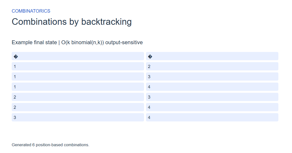
Step 25: Generated 6 position-based combinations.
State at this checkpoint
{
  "values": [
    "�",
    "�",
    1,
    2,
    1,
    3,
    1,
    4,
    2,
    3,
    2,
    4,
    3,
    4
  ],
  "active": [],
  "kind": "matrix",
  "columns": 2,
  "result": 6,
  "output": [
    1,
    2,
    1,
    3,
    1,
    4,
    2,
    3,
    2,
    4,
    3,
    4
  ]
}
Expected final state
Generated 6 position-based combinations.
Complexity and input bounds
Family: Combinatorics. Time complexity: O(k binomial(n,k)) output-sensitive.
Implementation detail: Inputs have at most seven positions and k from zero through n. Downloads return binomial(n,k) and write k values per row in lexicographic index order, preserving the original value order. Capacity k*binomial(n,k) is at most 140.
Space complexity: O(k) traversal state excluding output; Python retains generated rows. Saved visualization frames add space.
Working-space bounds describe algorithm state and any explicitly noted output, excluding the visualization's saved timeline. Recording frames can use more memory than running the function alone. Here n is sequence length, V and E are vertex and edge counts, and other parameters refer to the named input dimensions.
1..7 values 0..99 | k from 0 to n. Equal values at different positions remain distinct choices.
The playground validates these limits before starting. Downloaded functions are callable implementations, with parameter and output-buffer contracts in their comments; they do not all repeat the playground's input validation.
Common mistakes and limitations
Do not sort away positional semantics or deduplicate equal-valued rows. k zero has one empty combination; k equal to n has one complete combination.
Further reading
For background on algorithm analysis and the JavaScript function interface:
- MIT OpenCourseWare: algorithm design and analysis foundations
- MDN: JavaScript function parameters and return values
Editorial and testing approach · Browse all algorithm guides
Complete JavaScript implementation
1 2 3 4 5 6 7 8 9 10 | // n 0..7 values 0..99, k 0..n. Enumerates increasing-index combinations in lexicographic index order, preserving original input order. Duplicate values at distinct positions are separate choices. Returns binomial(n,k); writes k values per row, capacity at least k*binomial(n,k), at most 140. k=0 gives one empty result and writes nothing. O(k*binomial(n,k)) output work, O(k) traversal scratch excluding output; bounded branches are pruned. Reference snippets assume validated playground inputs. Fixed scratch buffers have 256 slots. Sorting variants may use a different traversal strategy than the animation. function algorithm(a, n, k, output) { if (k == 0) { return 1; } let chosen = Array(256).fill(0); let next = Array(256).fill(0); let depth = 0; let count = 0; let candidate = 0; while (depth >= 0) { if (depth == k) { for (let j = 0; j < k; j++) { output[count*k+j] = a[chosen[j]]; } count++; depth--; } else { candidate = next[depth]; if (candidate > n-(k-depth)) { depth--; } else { chosen[depth] = candidate; next[depth] = candidate+1; depth++; if (depth < k) { next[depth] = candidate+1; } } } } return count; } |
Source
Author reference for combinatorial generation, not a claim to an original research paper. The playground specifies its own bounded enumeration order and duplicate/position semantics.
- The Art of Computer Programming, Volume 4A: Combinatorial Algorithms, Part 1
Donald E. Knuth (2011). Author reference book.